Pore-scale viscous fingering as a mechanism for pattern formation – a historical overview, application, and the ways of controlling it

Figures & data

Figure 1. (a) The Kelvin-Helmholtz instability [7]; (b) from left to right, viscous, gravitational and inertial coiling respectively [8]; (c) the Rayleigh–Taylor instability [9]; (d) wine tears [10]; (e) and (f) immiscible [11] and miscible [12] viscous fingering, respectively.

Figure 2. Viscous fingering in Hele-Shaw cell with a planar channel geometry (a) and radial geometry (b).

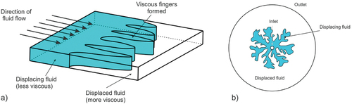
Figure 3. Oil recovery during the secondary and tertiary phases without and with the presence of viscous fingering (a comparison of displacement front stability). Adapted from [69].

Figure 4. MR (Magnetic resonance) signal intensity with flow rate 0.03 ml/min, pressure 6MPa and temperature 295 K shows the displacement process in quartz glass sands BZ-02. The CO₂ distribution is uneven prior to breakthrough, however, the displacement achieves a balance after some time, thus stabilizing the water and CO₂ distribution [78].

Figure 5. Model of growing tumour and invading neighbouring tissue; Adapted from [87].

Figure 6. Cross sections of the flat convergent (a) and divergent (b) Hele-Shaw cells [106]; Spherical (c) and conical (d) Hele-Shaw cell. Adapted from [107].

Figure 7. The Hele-Shaw flow in a planar channel geometry within the frame of reference.

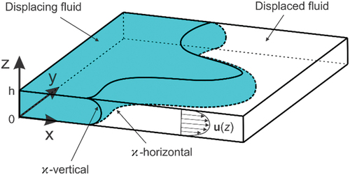
Figure 8. Expanding air bubble displacing the fluid between the plates (left) and velocity profile (right).

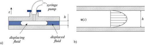
Figure 9. A perturbed interface in a radial flat rigid wall Hele-Shaw cell; Adapted from [119].

Figure 10. A complex bifurcation pattern of viscous fingering simulated by the DLA model; the patterns’ ages are indicated by their colours, with the first generated region being blue and the newly formed being red [132].

Figure 11. Schematic diagram of an elasto-rigid Hele-Shaw cell: a narrow gap between a rigid horizontal top plate and an elastomer confined within a rigid mould (left); fluid injected into the compliant Hele-Shaw cell at a constant flow rate spreads outwards, with a radial front position $r_f$, deforming the elastomer and displacing fluid resident in the cell; Adapted from [168].

Hydrodynamically unstable displacement ($\mathit{M}<1$) can be stabilized by electrokinetic control; an electro-osmotic flow can be stabilized by a positive current (electrokinetic thinning), however, a negative current of the same magnitude makes the displacement front unstable, resulting in the finger patter of smaller wavelengths [175].

Maharana S, Sahu K, Mishra M. Reaction-induced Kelvin-Helmholtz instability in a layered channel flow. J Fluid Mech. 2023;955:A36. doi: 10.1017/jfm.2022.1061

 Web of Science ®Google Scholar

Habibi M. Coiling instability in liquid and solid ropes [ Doctoral thesis]. Université Pierre et Marie Curie - Paris VI; 2007.

 Google Scholar

Fleishmann N, Adami S, Adams N. Numerical symmetry-preserving techniques for low-dissipation shock-capturing schemes. Comput Fluids. 2019;189:94–107. doi: 10.1016/j.compfluid.2019.04.004

 Web of Science ®Google Scholar

https://www.foodandwine.com/wine/wine-legs-tears-science

 Google Scholar

Sabet N, Mohammadi M, Zirrahi AZM, et al. Numerical modelling of viscous fingering during miscible displacement of oil by a paraffinic solvent in the presence of asphaltene precipitation and deposition. Int J Heat & Mass Trans. 2020;154:119688. doi: 10.1016/j.ijheatmasstransfer.2020.119688

 Web of Science ®Google Scholar

Pihler-Puzovic D, Juel A, Heil M. The interaction between viscous fingering and wrinkling in elastic-walled hele-Shaw cells. Phys Fluids. 2014;26:022102. doi: 10.1063/1.4864188

 Web of Science ®Google Scholar

Fanchi JR. Rock–fluid Interactions; integrated reservoir asset management. Boston: Gulf Professional Publishing; 2014. p. 167–185.

 Google Scholar

Jiang L, Song Y, Liu Y, et al. Magnetic resonance Imaging of CO2/Water two phase flow in Porous media. Energy Procedia. 2013;37:6839–6845. doi: 10.1016/j.egypro.2013.06.616

 Google Scholar

Bogdan MJ, Savin T. Fingering instabilities in tissue invasion: an active fluid model. R Soc Open Sci. 2018;5:181579. doi: 10.1098/rsos.181579

 PubMed Web of Science ®Google Scholar

Anjos PHA, Dias EO, Miranda JA. Fingering instability transition in radially tapered Hele-Shaw cells: insights at the onset of nonlinear effects. Phys Rev Fluids. 2018;3:124004. doi: 10.1103/PhysRevFluids.3.124004

 Web of Science ®Google Scholar

Brandão R, Fontana JV, Miranda JA. Suppression of viscous fingering in nonflat Hele-Shaw cells. Phys Rev E. 2014;90. doi: 10.1103/PhysRevE.90.053003

 Web of Science ®Google Scholar

Vaquero-Stainer C, Heil M, Juel A, et al. Self-similar and disordered front propagation in a radial Hele-Shaw channel with time-varying cell depth. Phys Rev Fluids. 2019;4:064002. doi: 10.1103/PhysRevFluids.4.064002

 Web of Science ®Google Scholar

Halsey TC. Diffusion-limited aggregation: a model for pattern formation. Phys Today. 2000;53:36–41. doi: 10.1063/1.1333284

 Web of Science ®Google Scholar

Box F, Peng GG, Pihler-Puzovic D, et al. Flow-induced choking of a compliant Hele-Shaw cell. Proc Natl Acad Sci, USA. 2020;117:30228–30233. doi: 10.1073/pnas.2008273117

 PubMed Web of Science ®Google Scholar

Gao T, Mirzadeh M, Bai P, et al. Active control of viscous fingering using electric fields. Nat Commun. 2019;10:4002. doi: 10.1038/s41467-019-11939-7

 PubMed Web of Science ®Google Scholar