Figures & data
Figure 1. (a) Snapshots of top view of Lallubhai Compound, Natwar Parekh Compound and PMG Colony. Study area of the three resettlement colonies is highlighted. Source: Google Earth, accessed on 20 June 2018. (b) Photographs of the open spaces between buildings in the three colonies (Source: Doctors For You, India)
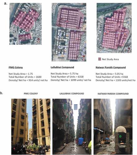
Table 1. Survey data used for correlation analysis
Table 2. Summary of boundary conditions used for natural ventilation simulation
Table 3. Sky view factor and air velocity in the three colonies calculated from simulation experiments
Table 4. Results of the simulation experiments for the three resettlement colonies
Figure 2. Change in DA of building with and without surrounding buildings in Lallubhai Compound (a), Natwar Parekh Compound (b) and PMG colony (c). Single building model – a computational model where a building was isolated in space from all other artefacts, so that light and air are accessible from all floors and all sides of the building. Urban model – a computation model where the building to be studied was considered to be surrounded by identical buildings on all sides as exists in the real scenario, according to the actual layout of the colony
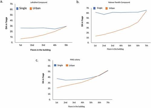
Figure 3. Volume rendering of air velocity within a typical room in Lallubhai Compound (a), Natwar Parekh Compound (b) and PMG colony (c). The color scheme should be read as follows: Red describes higher air velocity values and blues depicts velocities zero or near zero
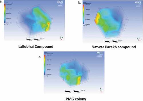
Figure 4. Air velocity profile of some representative tenements in Natwar Parekh Compound. Note: X-axis indicates building numbers and house numbers, e.g. 1A denotes ‘A’ wing of building number 1, whereas, 306 denotes 6th house on 3rd floor in that building
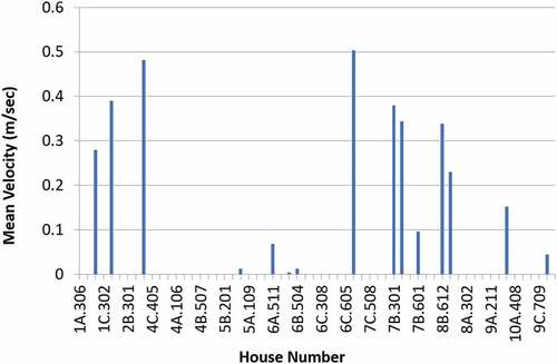
Figure 5. Income-wise distribution of tuberculosis patients
Figure 6. Time lapse between shifting to the colonies and occurrence of TB in the household in the three colonies. The X-axis shows difference between the time (in years) the patient caught the infection and the time he/she shifted to the colony, i.e. X = Year of TB infection – Year of Shifting to the colony. Positive values indicate that the person was infected after shifting into the colony, whereas negative values indicate that the person was infected before shifting into the colony. The zero value means that the year of shifting to the colony and year of infection with TB coincided for those particular patients. Note: These are taken from the self-reports of the patients from their own memory
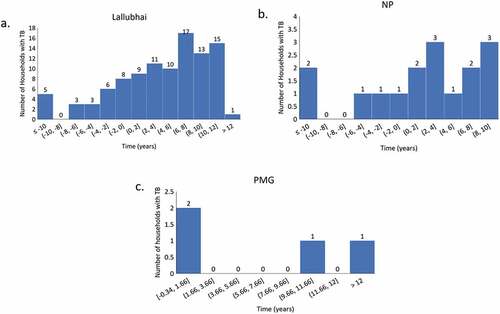
Table 5. Statistical analysis of model parameters
Figure 7. Age-wise distribution of tuberculosis patients
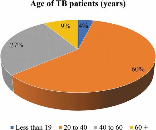
Table 6. Comparison of DCR for SRA and general buildings
Table 7. Comparison of layout of buildings for the three SRA colonies studied in the current article
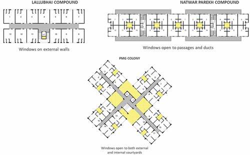
Figure 8. Floor plans of the three colonies