
Figures & data
Figure 1. Expectations for species occupancy given different tolerances to fragmentation (patch size) and habitat loss (amount of forest cover). If Polylepis specialists are adapted to patchy configurations of Polylepis forest, they are expected to be unrelated or less sensitive to patch size reduction (dashed line) (a-b), but either negatively affected by the reduction of amount of forest (solid line) (a) or unaffected by both (b). If not, Polylepis bird species are expected to be equally affected by patch size and forest loss (c). In contrast, species associated with the Puna matrix would positively respond to reductions in patch size and amount of forest cover (d). Finally, a nonlinear effect will be supported by the interaction of these two covariates, such as when patch size only has an effect at low amounts of forest (e.g. <30%) and vise versa (e)
Figure 2. Map of the five valleys studied within Cordillera Blanca, Peru. A total of 59 patches were included, ranging from 0.01 ha to 200 ha (a). Diagram of the patch and landscape attributes measured in our study (b)
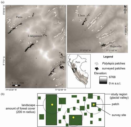
Figure 3. Examples of Polylepis forest from the glacial valleys of Ulta (a), Rajucolta (b), Llaca (c), Llanganuco (d) and Parón (e) within Cordillera Blanca. Matrix habitats are dominated by Puna grassland (a and e) or shrublands (f)
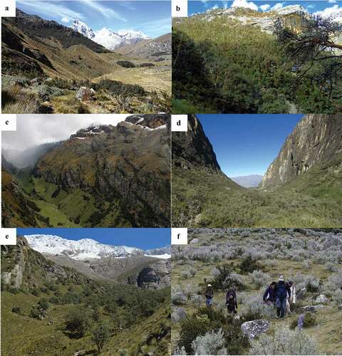
Figure 4. Contrasting predictions based on cumulative species-area curves, including (a) a positive association with patch size (i.e., samples in larger patches, while controlling for surveyed area, have more species), (b) negative association with patch size (i.e., more species in smaller patches), or (c) no association with patch size
Table 1. Community-level hyper-parameters for occupancy and detection in relation to elevation, patch size and amount of forest area. Each value represents the mean, standard deviation, and the 95% posterior interval of the effect of each parameter on the whole bird community. Rhat is the Brooks-Gelman-Rubin (BGR) measure of convergence of the three Markovian chains. Rhat <1.1 indicate convergence. These parameters correspond to our reduced model
Figure 5. Average (among three years) local species richness (alpha diversity) at each site (n=187) declines with increasing elevation (a), patch size (b) and amount of Polylepis forest within 200 m-radio (c). Black dots and vertical lines represent the average mean and 95% posterior intervals of the species richness estimated through MSOM for each site. The solid black and shade areas represent the mean ± 95% CI of lineal regressions
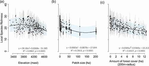
Figure 6. Avian community composition across five different categories of patch size and amount of forest cover within the landscape. The community was classified according to (1) habitat associations (a, b), (2) five foraging guilds (c, d), and (3) status of conservation priority (e, f). The total numbers of observations during the three years on each category are in parenthesis over each bar (this applies to the other two graphs below)
Figure 7. Mean community occupancy for birds in the High Andes was highest at mid-to-low elevations (a), in large forest patches (b) and in local landscapes with relatively low forest cover (c) while accounting for detectability per year (d,e,f). Shade areas represent the 95% of posterior intervals. Parameters y2 and y3 correspond to second- and third-year effect with respect to the initial year (α0) (f)
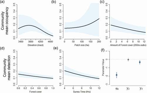
Figure 8. Species- and community- level responses to elevation (a-b), patch size (c-d) and amount of Polylepis forest cover in the landscape (e-f). Open dots represent the species-specific mean response. Horizontal lines represent the 95% posterior intervals. Intervals that do not overlap zero (blue lines) indicate that estimated coefficients differed significantly from zero, indicating an effect of the parameter. Solid and dashed vertical lines (red) are the mean and 95% PI of the community response, respectively. Species ID correspond those in Table S1
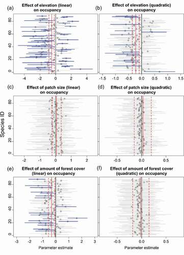
Figure 9. Mean species occupancy probabilities in response to Polylepis patch size (left in a,b,c,d) and amount of forest cover (%) within 200-m radio (right in a,b,c,d). The solid lines and shade areas represent the mean ± 95% Posterior Intervals of the reduced MSOM. Cobin = Giant Conebill, Crbar = Baron’s Spinetail, Atruf = Rufous-eared Brushfinch, Grand = Stripe-headed Antpitta, Lepil = Rusty-crowned tit-spinetail, Mepho = Black Metaltail, Mialt = Plain-tailed Warbling-Finch, Scaff = Ancash Tapaculo, Xepar = Tit-like Dacnis, Zastr = White-cheeked Cotinga, Ocruf = Rufous-breasted Chat-tyrant, Geser = Striated Earthcreeper. Individual plots of the 88 species are in Figure S7
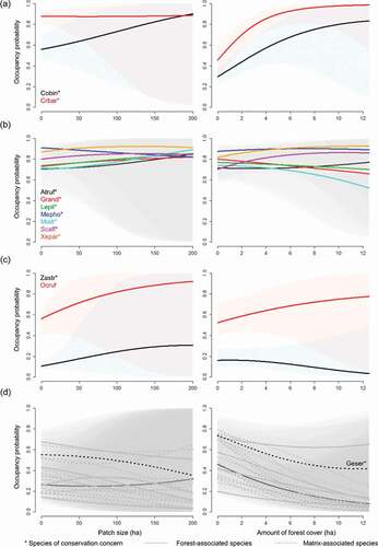
Figure 10. Species richness estimation across both orders (large to small and vise-versa) of cumulative forest area of 59 Polylepis surveyed patches for all (a), forest (b), grassland Puna (c) and shrubland (d) species. Shade lines correspond to the 95% confidence interval
Table 2. Proportion of forest cover with respect to the landscape extension of each of the five glacier valleys studied in Cordillera Blanca, Peru. The landscape extension was delimitated by the natural entrance of the valleys and the 5,000 m elevational line and calculated based on a Digital Elevation Model. The forest cover was calculated in the same way as the studied patches