
Figures & data
Figure 1. Photograph of burnt Polylepis microphylla shrubs in the study area
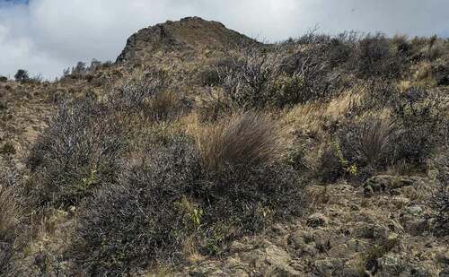
Figure 2. Tree habit of Polylepis microphylla of approximately 4 m high located in forest 1
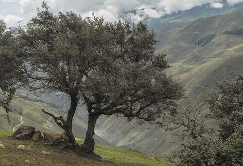
Figure 3. Detail of mature flower and leaves of Polylepis microphylla
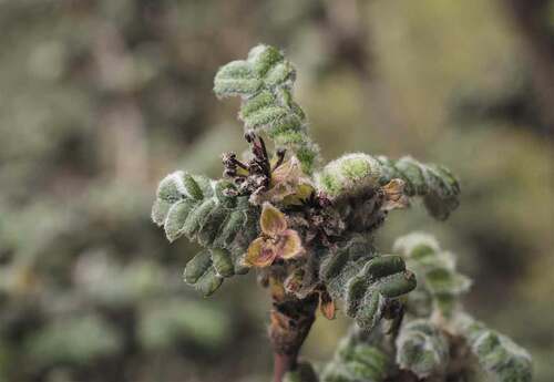
Figure 4. Map of two Polylepis microphylla forests in the study area in Chimborazo province, Ecuador
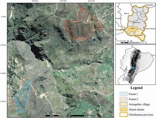
Figure 5. Photograph of forest 1. The open grassland area is dominated by agricultural activities where Polylepis microphylla grows
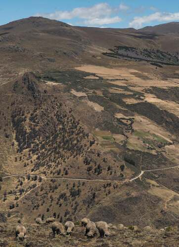
Figure 6. Photographs of forest 2. A) Polylepis microphylla represented by shrubs of maximum 1,5 m high. Area dominated by grassland. B) A slope of P. microphylla coverage
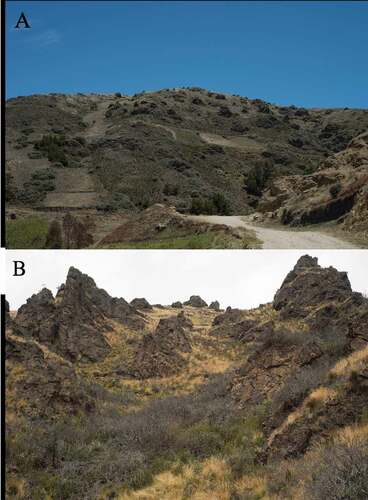
Table 1. DNA regions used. The type of region, primers used, their sources and temperatures of annealing (TA) are indicated
Table 2. Segregation sites and haplotype frequencies of trnG intron with their position in the final alignment and their frequencies in the two forests. (-) represents the same nucleotide in relation to the first sequence
Table 3. Segregation sites and haplotype frequencies of ITS region with their position in the final alignment and their frequencies in the two forests. (-) represents the same nucleotide in relation to the first sequence
Table 4. Segregation sites and haplotype frequencies of the concatenated regions with their position in the final alignment and their frequencies in the two forests. (-) represents the same nucleotide in relation to the first sequence
Table 5. Analysis of molecular variance (AMOVA) in trnG intron, ITS and concatenated regions in the two forests (P > 0,05). (d.f) degrees of freedom, (Va) Variance of components among forests, (Vb) Variance of components within forests, (Fst) Weir & Cockerham (1984) fixation index
Table 6. Genetic diversity estimators, distribution and frequency of haplotypes within and both forests in trnG intron, ITS and concatenated regions. (n) sample size; (S) number of segregation sites; (h): number of haplotypes; (hd) haplotype diversity; (π) nucleotide diversity, * represents unique haplotypes
Figure 7. Relationships of the 9 haplotypes generated from trnG intron represented by a median joining network. Each circle represents a different haplotype and the crossed lines represent nucleotide differences
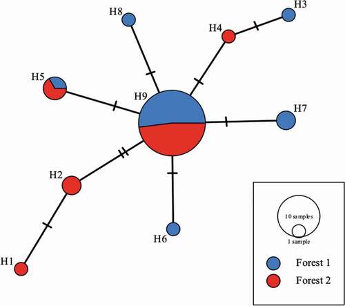
Figure 8. Relationships of the 6 haplotypes generated from ITS region represented by a median joining network. Each circle represents a different haplotype and the crossed lines represent nucleotide differences
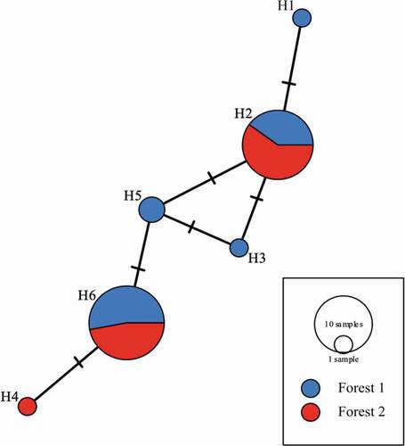
Figure 9. Relationships of the 15 haplotypes generated from the concatenated regions represented by a median joining network. Each circle represents a different haplotype and the crossed lines represent nucleotide differences. Median vector could be interpreted as an unsampled or extinct haplotype
