Plant community associations with morpho-topographic, geological and land use attributes in a semi-deciduous tropical forest of the Dominican Republic

Figures & data

Figure 1. Location map of 23 sampling sites (circles filled white), showing the town of San José de Ocoa (see a description of the rock/landform attributes of the sites in Table A1). The overlapping points are depicted slightly displaced from their actual positions to ensure that all become visible. The background is a color shaded-relief view (red-white is highland, green is lowland) based on a 30-m SRTM DEM (Ref: NASA LP DAAC, 2000. SRTM 1 Arc-Second Global, https://earthexplorer.usgs.gov/. Published September 2014). The bottom-left inset shows the area in the context of the Dominican Republic

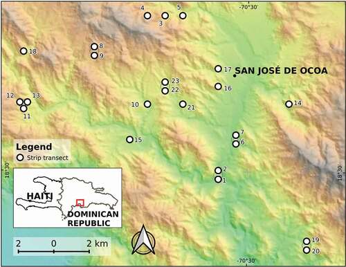
Figure 2. Dendrogram of groups of sites based on selected environmental variables. Groups are indicated by bold letters A to F, and sites are denoted by numbers. See text for details and Table A1 for a description of the transects

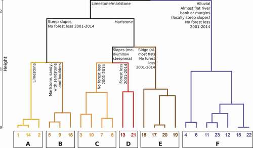
Table 1. IndVal calculations for 11 significantly associated species with groups of sites

Species	A	B	C	D	E	F	IndVal	p	Aind	Bpa
Acacia skleroxyla		X	X	X	X		0.952	0.006	0.981	0.923
Ateleia gummifera		X		X	X		0.818	0.049	0.861	0.778
Coccoloba incrassata				X	X		0.784	0.049	0.923	0.667
Eugenia foetida					X		0.909	0.016	0.827	1.000
Exostema caribaeum			X	X			0.874	0.007	0.916	0.833
Phyllostylon rhamnoides	X						0.816	0.035	1.000	0.667
Pictetia sulcata				X	X		0.801	0.039	0.962	0.667
Randia aculeata		X	X	X	X		0.978	0.002	0.956	1.000
Savia sessiliflora	X						0.718	0.049	0.772	0.667
Schaefferia frutescens		X					0.764	0.044	0.875	0.667
Trichilia pallida						X	0.839	0.022	0.821	0.857

Legend: Species: genus and species name in alphabetical order. A, B, C, D, E, F: “X” means IndVal shows that the species is associated to the group of sites. IndVal: indicator value index. p: p-values from permutation test to assess the significance of the association between species and groups of sites, summarizing the maximum p-value obtained from the different permutations sets (a conservative approach). A_ind: positive predictive value. B_pa: fidelity or sensitivity.

Table 2. R_pb calculations for 13 significantly associated species with groups of sites

Species	A	B	C	D	E	F	rpb	p
Ateleia gummifera				X			0.752	0.022
Coccoloba incrassata					X		0.696	0.048
Coccothrinax argentea				X			0.990	0.007
Eugenia foetida					X		0.796	0.009
Exostema caribaeum			X	X			0.727	0.032
Hura crepitans						X	0.694	0.046
Leucaena leucocephala				X			0.683	0.046
Phyllostylon rhamnoides	X						0.706	0.035
Picramnia pentandra						X	0.668	0.049
Pictetia sulcata				X	X		0.656	0.049
Samyda dodecandra				X			0.708	0.028
Schaefferia frutescens		X					0.703	0.045
Trichilia pallida						X	0.700	0.039

Legend: Species: genus and species name in alphabetical order. A, B, C, D, E, F: “X” means r_pb shows that the species is associated to the group of sites. r_pb stands for phi point-biserial correlation coefficient.

Table 3. List of species significantly associated with one or more groups of sites by means of IndVal and/or r_pb.

Species	IndVal	rpb
Acacia skleroxyla	X
Ateleia gummifera	X	X
Coccoloba incrassata	X	X
Coccothrinax argentea		X
Eugenia foetida	X	X
Exostema caribaeum	X	X
Hura crepitans		X
Leucaena leucocephala		X
Phyllostylon rhamnoides	X	X
Picramnia pentandra		X
Pictetia sulcata	X	X
Randia aculeata	X
Samyda dodecandra		X
Savia sessiliflora	X
Schaefferia frutescens	X	X
Trichilia pallida	X	X

Figure 3. Triplot of the Hellinger-transformed abundance community matrix, constrained by the variables (blue outlined rectangles) lithology, geomorphology, forest loss 2001–2014 and slope. Though we used the entire community matrix for computing the RDA, we only plotted the 16 species associated by means of IndVal and r_pb. This is a scaling 2 triplot, where angles between species and explanatory variables, and angles between species themselves and variables themselves, are interpreted as correlations. The labelled (A to F) ellipses with grey dotted border enclose site groups defined by the AGNES agglomerative hierarchical clustering algorithm. See text for details and Table A1 for a description of the transects

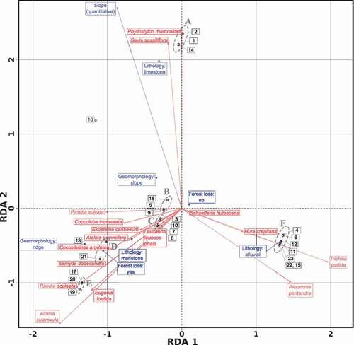
Table 4. Regression results from fitting the environmental variables onto a PCA ordination of a Hellinger transformed community matrix

Variable	r^2	Pr(> r)
Slope	0.188	0.136
Lithology	0.385	0.001
Geomorphology	0.265	0.009
Forest loss	0.071	0.264

Table A1. Morpho-topographic, geological and land use attributes of the transects

Site	Lithology	Geomorphology	Slope (radians)	Forest loss 2001–2014
1	Limestone	Slope	0.44	No
2	Limestone	Slope	0.58	No
3	Marlstone	Slope	0.32	No
4	Alluvial	River bank/margin	0.29	No
5	Marlstone w/ boulders+sand	Slope	0.44	No
6	Alluvial	River bank/margin	0.28	No
7	Marlstone	Slope	0.24	No
8	Marlstone	Slope	0.22	No
9	Marlstone w/ boulders+sand	Slope	0.42	No
10	Marlstone	Slope	0.29	No
11	Alluvial	River bank/margin	0.20	No
12	Alluvial	River bank/margin	0.22	No
13	Marlstone	Slope	0.36	Yes
14	Limestone	Slope	0.44	No
15	Alluvial	River bank/margin	0.16	No
16	Limestone	Ridge	0.27	No
17	Marlstone	Ridge	0.29	No
18	Marlstone w/ boulders+sand	Slope	0.55	No
19	Marlstone	Ridge	0.21	No
20	Marlstone	Ridge	0.29	No
21	Marlstone w/ boulders+sand	Slope	0.14	Yes
22	Alluvial	River bank/margin	0.16	No
23	Alluvial	River bank/margin	0.19	No

Legend: Lithology, rock types identified with field recognition and consultation of geological maps. Geomorphology, classified using field observation and aerial photography. Slope, average of a 5$\times$5 moving window centered on each site from a slope raster. Forest loss 2001–2014, based on high-resolution global maps and subsequent updates [see 27,28].

Hansen MC, Potapov PV, Moore R, et al. High-resolution global maps of 21st-century forest cover change. science. 2013;342(6160):850–853.

 PubMed Web of Science ®Google Scholar

Hansen MC, Potapov PV, Moore R, et al. Global forest change; 2015. Available from: http://earthenginepartners.appspot.com/science-2013-global-forest

 Google Scholar