Figures & data
Table 1. Kruskal–Wallis test the influence of depth range sampling conditions on abundance, species richness and diversity of copepods in offshore waters of Colombian Caribbean. ** = Highly significant (P < 0.001). N: Abundance (ind. 100 m−3), S: Richness, H’: Shannon diversity index, J’ = Pielou uniformity index and Lambda’: Simpson dominance index
Figure 1. Study area in the Colombian Caribbean Sea with the location of the zooplankton sampling stations for the years 2013–2018
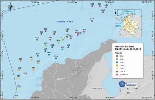
Figure 2. Species accumulation curve of copepods with Chao2, Jacknife2, Bootstrap and Sobs in the samples obtained in oceanic waters of Colombian Caribbean during 2013–2018
Figure 3. Ecological attributes and morphological characters of the copepod assembly found in ocean waters of the Colombian Caribbean. Percentage of species by a. Vertical distribution: Bathypelagic (Bat), Epipelagic (Epi), Mesopelagic (Meso); b. Habitat distribution: Coastal (C), Estuarine (E), Neritic (N), Oceanic (O); c. Trophic regime: Herbivorous (Herb), Omnivorous (Omn), Detritivorous (Detri), Carnivorous (Carn); d. Size spectrum: millimeters (mm)
Figure 4. Funnel plot for simulated average taxonomic distinction Delta+ (AvTD = Δ+) (a) and for variation in taxonomic distinctness Lambda+ (VarTD = Ʌ+) (b) of epipelagic and mesopelagic copepods in four depth range (0–60 m, 70–140 m, 170–340 m and 540–1000 m) in the Offshore Caribbean Sea. “ – –” shows average and “_____” show probability distribution at 95%
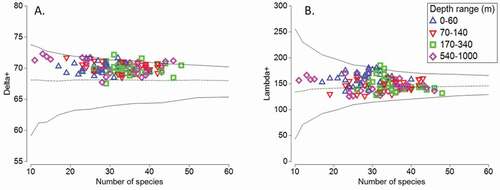
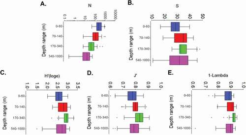
Figure 5. Box and whiskers plot of abundance, richness and the diversity indices in four depth range (0–60 m, 70–140 m, 170–340 m and 540–1000 m) for the assemblage of epipelagic and mesopelagic copepods found in the CAO ecoregion between the years 2013 and 2018. a. N = species density (ind.m3), b. S = species richness, c. H’ = Shannon loge diversity index, d. J’ = Pielou species evenness index, e. 1 -Lambda = Simpson dominance index