Investigations of accelerated methods for determination of chloride threshold values for reinforcement corrosion in concrete

Figures & data

Table 1. Mix proportions.

Ingredients	Specimens from ETH	Specimens from DTI
(kg/m^3)	(kg/m^3)	(kg/m^3)
Portland Cement	330 (CEM I 42.5 N – Normo 4 – Holcim)	380 (CEM I 42.5 N – SR 5 – Aalborg Portland)
Water (w/c-ratio 0.5)	165	189.1
Aggregate (0–4 mm)	756	793 (0–2 mm sand)
Aggregate (4–8 mm)	567	984
Aggregate (8–16 mm)	567	-
Superplasticizer	-	1.2
Curing	4 weeks at 20°C and 95% RH (climate chamber)	All specimens were demoulded after seven days and subsequently left for curing under plastic sealing for further 21 days in the laboratory (approx. 20°C)
Steel type/ surface preparation	Ø12 mm, B500B, ferritic-pearlitic As-received conditions	Ø10 mm S235JR (EN 10,025) Chemically cleaned by immersion in a chemical cleaner solution (HCl:H2O = 1:1 + 3 g/l urotropine) for 5 minutes and subsequent treatment in an ultra-sonic bath for 3 minutes

Figure 1. Schematic illustrations of the specimen designs used at ETH (a) and DTI (b).

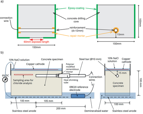
Figure 2. Different exposure methods tested: a) diffusion D b) wetting/drying WD, c) migration 1 M1, d) migration 2 M2, and e) migration M3 and M4. Table 2 gives an overview of the tested methods for chloride ingress.

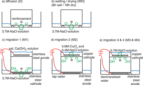
Table 2. Summary of applied techniques for chloride ingress.

method	number of parallel specimens	chloride ingress (primary mechanisms indicated)	applied current density (A/m^2) with respect to concrete surface area	remarks
diffusion D	4	diffusion	-	-
wetting/drying WD	3	capillary suction & diffusion	-	6 h wet/18 h dry
migration 1 M1	6	migration	0.05–0.52	-
migration 2 M2	3	migration	0.05–0.4	-
migration 3 M3	4	migration	not measured (6 V applied across the sample)	-
migration 4 M4	2	migration (and diffusion)*	not measured (6 V applied across the sample)	-

*The chloride ingress was driven by a combination of migration and diffusion for two of the six investigated specimens, since the external DC voltage was switched off for a prolonged period before initiation of corrosion was detected.

Figure 3. Current densities used for M1 and M2.

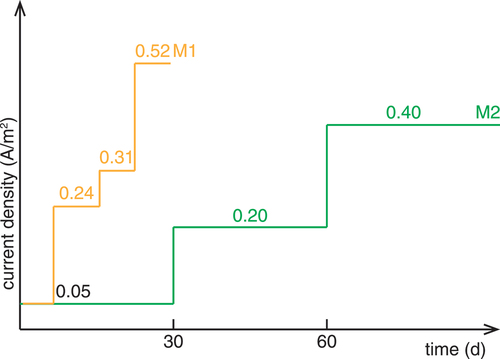
Figure 4. Example of measured steel potentials vs. time in experiments at DTI with method M3. Only ‘off’ potentials are shown in the figure, i.e. potentials measured during the periods with applied DC voltage (6 V) has been filtered out. The potential drop observed after about 14 days indicates the onset of corrosion in this particular specimen (‘7_15 mm’). The potentials are measured with an Mn/MnO₂ reference electrode but corrected to mV vs. Ag/AgCl_sat by addition of 222 mV.

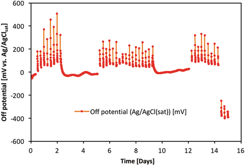
Figure 5. Schematic illustration showing the duration of periods, where the DC voltage (6 V) was only switched off at regular intervals (four times a day) for 1 hour to observe the ‘off’ potential of the steel (continuous, red lines), and periods where the DC voltage was switched off manually (dotted, blue lines). This is shown for both method M3 (a) and M4 (b). A summary of the total time for each DTI specimen, where the DC voltage was turned on and off during the experiments is given in Table 3. For interpretation of the references to color in this figure legend, the reader is referred to the web version of this article.

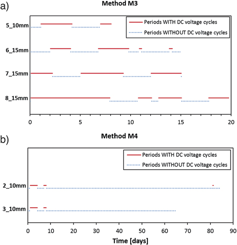
Table 3. Overview of total time with and without applied DC voltage in the experiments with method M3 and M4.

Method	Specimen ID	Total time with DC voltage turned ON during testing	Total time with DC voltage turned OFF during testing
		(d)	(d)
M3	5_10 mm	3.5	4.4
	6_15 mm	4.9	10.1
	7_15 mm	7.6	7.5
	8_15 mm	11.3	8.5
M4	2_10 mm 3_10 mm	3.8 3.6	80.2 61.4

Figure 6. Time to corrosion initiation for the different testing conditions (note that for reasons of comparison, only samples with equal cover depth (15 mm) are shown here). For interpretation of the references to color in this figure legend, the reader is referred to the web version of this article.

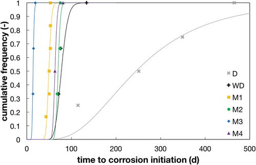
Table 4. Time to corrosion initiation and C_crit for different accelerating methods. (µ = mean value, $\sigma$ = standard deviation).

Method(-)	Cover depth (mm)	Time to corrosion initiation (d)	Ccrit (% by cem.wt.)
Diffusion D	15	115; 251; 349; 465 µ: 295; $\sigma$: 129	1.37; 2.04; 2.12; 3.06 µ: 2.16; $\sigma$: 0.61
wetting/drying WD	15	71; 76; 134 µ: 94; $\sigma$: 29	0.98; 1.64; 2.13 µ: 1.58; $\sigma$: 0.47
migration 1 M1	15	43; 50; 50; 53; 53; 53 µ: 50; $\sigma$: 4	0.65; 1.04; 1.08; 1.25; 1.33; 1.65 µ: 1.17; $\sigma$: 0.3
migration 2 M2	15	68; 74; 75 µ: 72; $\sigma$: 3	1.22; 1.35; 1.41 µ:1.33; $\sigma$: 0.08
migration 3 M3	10	8	1.66
	15	14; 15; 19 µ: 16; $\sigma$: 2.40	1.34; 1.59; 1.98 µ: 1.64; $\sigma$: 0.26
migration 4 M4	10	63; 81 µ: 72; $\sigma$: 9	2.47; 3.02 µ: 2.75; $\sigma$: 0.28

Figure 7. Box Plots of the C_crit values for the different methods. The horizontal lines of the boxes represent the 25%, 50%, and 75%-quantiles. The whiskers are the extreme values. Number of specimens per series is D: 4, WD:3, M1: 6, M2: 3, M3: 4 (both cover layers were combined), and M4: 2 (according to Table 2).

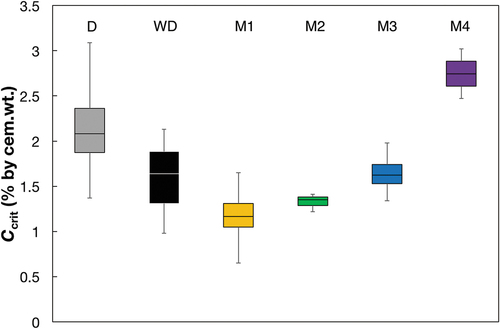
Figure 8. C_crit vs. time to corrosion initiation, distinguished by acceleration techniques. (note that for reasons of comparison, only samples with equal cover depth (15 mm) are shown here).

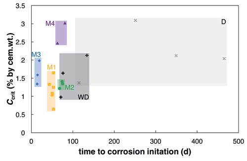
Figure 9. Box plots of potentials before (a) and after (b) initiation of corrosion. The horizontal lines of the boxes represent the 25%, 50%, and 75%-quantiles. The whiskers are the extreme values. Number of specimens per series is D: 4, WD:3, M1: 6, M2: 3, M3: 4 (both cover layers were combined), and M4: 2 (according to Table 2).

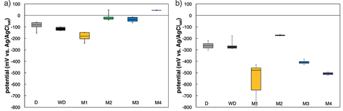
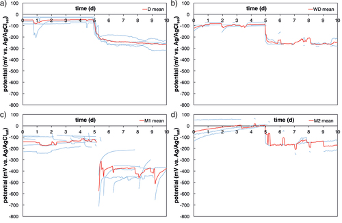
Figure 10. Potential vs. time, 5 days before and 5 days after initiation of corrosion (potential drop > 150 mV). a) is method D, b) method WD, c) method M1, and d) method M2. The red line depicts the mean value, the thin blue lines depict each sample. For interpretation of the references to color in this figure legend, the reader is referred to the web version of this article.