Developing adaptive resilience in infrastructure systems: an approach to quantify long-term benefits

Figures & data

Figure 1. Resilience triangle (Bruneau et al.2003).

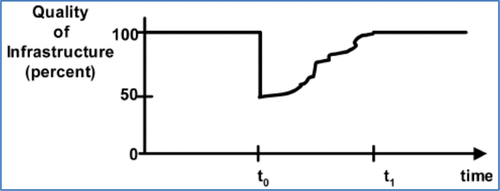
Figure 2. Seismic resilience triangle assessment comparing Oregon and Japan’s resilience (Yu et al., 2014).

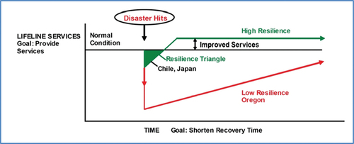
Figure 3. Resilience loss triangle for supply chain (Sheffi & Rice, 2005).

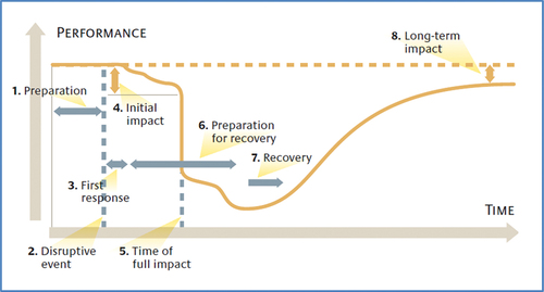
Figure 4. Resilience loss changes with different adaptive resilience strategy directions.

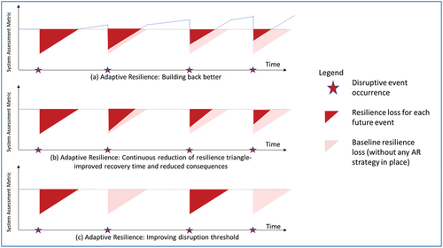
Table 1. MRT assessment steps- input.

1	Resilience Strategy(i)	CAEP | (RS0 … … RSn)
2	Context-specific performance measure (Q)	Essential Services Availability Index (ESAI)
3	Time period of assessment	50 years
4	RL(i) calculation	[See the results section]
5	RL(i,T)	RL4 as a function of time – linear improvement every 10 years from RL1 to RLn over the LC
6	f(T)	Population (future projections based on census data)
7	Scenarios (k)	K = {1,2,3}: SLR – Low, SLR – low-intermediate, SLR – Intermediate-High (based on IPCC)
8	Disruption Parameter	Hurricane Wind Speed
9	GEV parameters	[See, Table 2]
10	Disruption threshold	96 knots (Hurricane category 3 wind speed)
11–14	Results Calculation	[See the results section]

Table 2. GEV parameters for the different SLR scenarios.

	GEV parameters
Scenario	Location (µ)	Scale (σ)	Shape (ξ)
Baseline- Low SLR	64	36	−0.37
Low-Int SLR	66.47	36	−0.37
Int-High SLR	69.09	36	−0.37

Figure 5. Resilience triangle for different RL cases- CAEP.

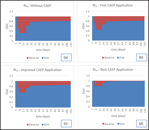
Figure 6. Expected resilience loss for each year in the assessment timeframe for each SLR scenario – CAEP.

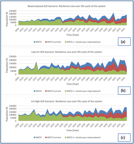
Figure 7. Total expected resilience loss over the time period of the assessment for each SLR scenario, and the expected RL across all scenarios.

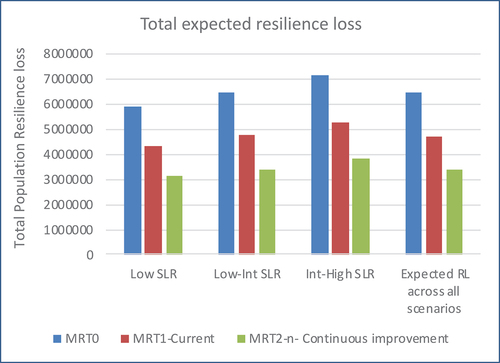
Table 3. MRT assessment steps: data inputs for transitgrid.

1	Resilience Strategy(i)	TransitGrid | (RS0, RS1, RS2)
2	Context-specific performance measure (Q)	Transit Functionality Score (TFI)
3	Time period of assessment	50 years
4	RL(i) calculation	[see the results section]
5	RL(i,T)	RL2 as a function of time – first potential improvement at year 10, constant thereafter
6	f(T)	Rail miles (expansion of rail miles over time- NJ Transit data)
7	Scenarios (k)	K = {1,2,3}: SLR – Low, SLR – low-intermediate, SLR – Intermediate-High (based on IPCC)
8	Disruption Parameter	Hurricane Wind Speed
9	GEV parameters	[see, Table 4]
10	Disruption threshold	96 knots (Hurricane category 3 wind speed)
11–13	Results Calculation	[see the results section]

Table 4. GEV parameters for NJ hurricane wind speeds.

	GEV parameters
Scenario	Location (µ)	Scale (σ)	Shape (ξ)
Baseline- Low SLR	77.2	10.6	−0.0544
Low-Int SLR	79.49	10.6	−0.0544
Int-High SLR	83.25	10.6	−0.0544

Figure 8. Resilience loss for different cases of transitgrid application.

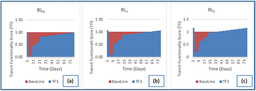
Figure 9. Expected resilience loss for each year in the assessment timeframe for each SLR scenario -Transitgrid.

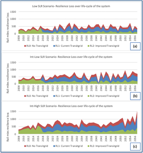
Figure 10. Total expected resilience loss over the timeframe of the assessment for each SLR scenario, and the expected RL across all scenarios – Transitgrid.

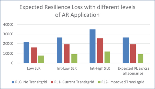
Table 5. MRT assessment inputs: Tex-Wash Bridge.

1	Resilience Strategy(i)	Bridge Flood Management | (RS0, RS1, RS2, RS3, RS4)
2	Context-specific performance measure (Q)	Economic benefit of the bridge ($)
3	Time period of assessment	90 years
4	RL(i) calculation	[See the results section] All RL(i) have the same value
5	RL(i,T)	-
6	f(T)	Time value of money – discount rate of 5%
7	Scenarios (k)	K = {1,2}: Two future projection models – CNRM-C5 (Cooler/Wetter), and HadGEM2-ES(Warm/Drier)
8	Disruption Parameter	Max daily precipitation
9	GEV parameters	Calculated using projection models
10	Disruption threshold	Variable with each strategy [see, Table 7]
11–13	Results Calculation	[See the results section]

Table 6. DAP triggers and improved thresholds.

Trigger	Action	Improved threshold
Trigger 0: 100-yr return level projected 20 years from time (T) is less than 6 inches	No action	6 inches
Trigger 1: 100-yr return level projected 20 years from time (T) is between 6–8 inches	Deck rehab (raising/strengthening)	8 inches
Trigger 2: 100-yr return level projected 20 years from time (T) is between 8–10 inches	Deck replacement	10 inches
Trigger 3: 100-yr return level projected 20 years from time (T) is between 10–12 inches	Deck replacement+ superstructure & substructure rehab	12 inches
Trigger 4: 100-yr return level projected 20 years from time (T) is greater than 12 inches	bridge replacement	14 inches

Table 7. Thresholds for static resilience strategies.

Resilience Strategy	CNRM-CM5 Model	HadGEM2-ES Model
RS0 (Build back same)	6 inches	6 inches
RS1(mid-century plan)	8.23 inches	7.09 inches
RS2(end-century plan)	10.25 inches	8.37 inches

Figure 11. Resilience loss triangle for bridge closure\Tex-Wash Bridge.

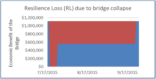
Figure 12. Expected resilience loss for each year in the assessment timeframe for each SLR scenario -Tex Wash Bridge.

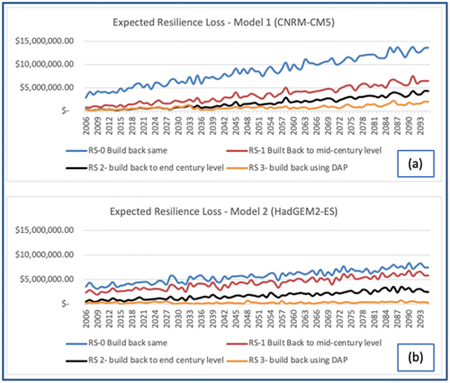
Figure 13. Total expected resilience loss over the time period of the assessment for each SLR scenario, and the expected RL across all scenarios – Tex Wash Bridge.

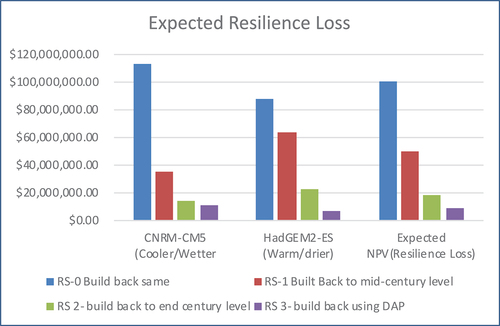
Table 8. Percentage reduction in expected resilience loss with different AR strategies across all considered scenarios.

CAEP		TransitGrid		Tex-Wash Bridge DAP
-	-	-	-	RL1- Built Back to mid-century level	51%
RL1-Current CAEP	27%	RL1-Current TransitGrid	27%	RL2- build back to end century level	82%
RL2- Continuously Improved CAEP	48%	RL2- Improved TransitGrid	66%	RL3- build back using DAP	92%

Bruneau, M., Chang, S. E., Eguchi, R. T., Lee, G. C., O'Rourke, T. D., Reinhorn, A. M.,& Von Winterfeldt, D. (2003). A framework to quantitatively assess and enhance the seismic resilience of communities. Earthquake spectra, 19(4), 733-752.

 Google Scholar

Yu, K., Wilson, J., & Wang, Y. (2014). 10th US National Conference on Earthquake Engineering, July 2014, Alaska. doi:10.4231/D3CN6Z08T.

 Google Scholar

Sheffi, Y., & Rice, J. (2005). A supply chain view of the resilient enterprise. MIT Sloan Management Review, 47. https://sloanreview.mit.edu/article/a-supply-chain-view-of-the-resilient-enterprise/.

 Web of Science ®Google Scholar