
Figures & data
Table 1. Basic features of the plastomes of ten Photinia species.
Figure 1. Graphic representation of features identified in P. davidsoniae plastome. The map was created with CPGAVAS2. Counted from the center, the first circle shows the forward and reverse repeats. They are connected with red and green arcs, respectively. The second and third circles indicate the locations of the tandem repeats and microsatellite sequences represented with short bars. The fourth circle shows the positions of plastome genes. The genes are colored base on their functional categories.
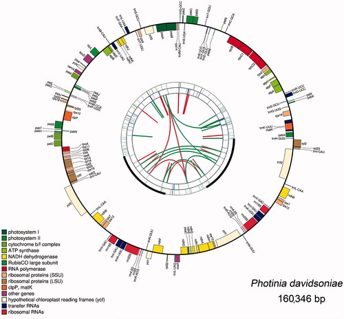
Table 2. Gene contents of the plastomes of Photinia species.
Figure 2. Comparison of the Repeats in the plastomes of Photinia species. (A) Types and numbers of SSRs detected in the plastomes of ten Photinia species; (B) Types and numbers of tandem repeats and dispersed repeats detected in the plastomes of ten Photinia species.
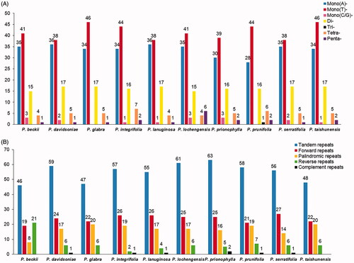
Figure 3. Comparison of LSC, SSC, and IR border regions of species from Photinia and related genera. The genes around the borders are shown above or below the mainline. The JLB, JSB, JSA, and JLA represent junction sites of LSC/IRb, IRb/SSC, SSC/IRa, and IRa/LSC, respectively. ‘*’: pseudogene.
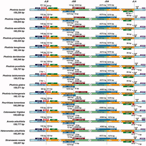
Figure 4. Comparison of the cp genomes in Photinia species by using mVISTA. The gray arrows on the top of the alignment represent genes. The pink regions are ‘Conserved Non-Coding Sequences’ (CNS), the dark blue regions are exons, and the light-blue regions are tRNA or rRNA. The percentages (50% and 100%) are the similarity among these sequences. Gray arrows on the top of the aligned sequences represent genes and their orientation. The colored lines under each window represent different regions of the plastomes: the blue line refers to the LSC region, the red line refers to the IR regions, and the green line refers to the SSC region.
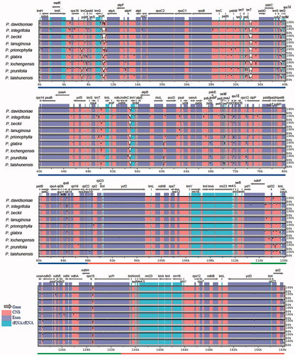
Figure 5. Hypervariable regions in Photinia species. We used a sliding window to analyze the sequence polymorphism among the plastomes of ten Photinia species. The sliding window has a length of 600 bp and a step size of 200 bp. The X-axis represents the position of nucleotide; Y-axis represents nucleotide polymorphism of each window.
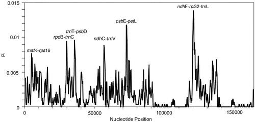
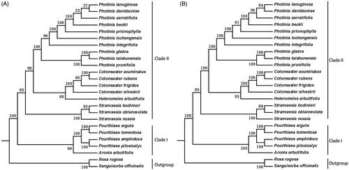
Figure 6. Phylogenetic relationships of species from Photinia and related genera inferred using the Maximum likelihood (ML) method. A. The phylogenetic tree was constructed was constructed using the complete nucleotide sequences of the using the 75 common protein sequences among the 25 cp genomes. B. The phylogenetic tree 25 cp genomes. Two taxa, namely, R. rugosa and S. officinalis, were used as outgroups. Bootstrap values were calculated from 1000 replicates.
Data availability statement
The sample has been deposited in the herbarium of the Institute of Medicinal Plant Development in Beijing, China, with the accession number: implad201808128. The genome sequence data that support the findings of this study are openly available in GenBank of NCBI at (https://www.ncbi.nlm.nih.gov/) under the accession no. MT230547. The associated BioProject, Bio-Sample, and SRA numbers are PRJNA688534, SAMN17180600, and SRR13325884, respectively.