Figures & data
Table 1. Mitogenome sequences were used in this study.
Figure 1. The graphical visualization of Otus lettia mitogenome.
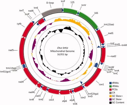
Figure 2. The base composition (a) and A + T content (b) of 29 Strigiformes mitogenomes. Each circle represents a mitogenome.
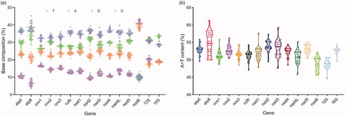
Figure 3. Statistics of variation sites (a), nucleotide diversity (b), Ka (c), Ks (d), and Ka/Ks (e) of 29 Strigiformes mitogenomes.
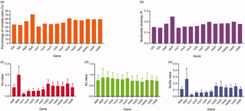
Figure 4. Alignment of the mitochondrial nad3 gene region spanning the extra cytosine insertion for Strigiformes species. Additional three nad3 sequences EU601009, MN356151, and EU601014 were used to show the intraspecific differences of inserted cytosine.
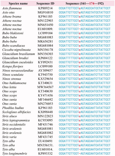
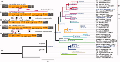
Figure 5. Strigiformes mitochondrial gene arrangement types (a) and BI and ML phylograms inferred from 10 PCGs and two rRNAs (b). The orders of the genes outside the region depicted in this figure are the same. The phylograms were visualized and annotated using FigTree (http://tree.bio.ed.ac.uk/software/figtree/). Values at nodes are Bayesian posterior probabilities, SH-aLRT bootstrap percentages, and ultrafast bootstrap percentages, respectively. I–IV denote five different gene arrangement types. ‘?’: the arrangement type is uncertain due to incomplete sequencing.