Figures & data
Figure 1. Conceptual computational radiology framework for personalized radiological diagnosis and prognosis. There are three major components of the proposed framework – image segmentation, feature extraction and integrated clinical decision support model.
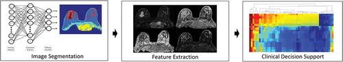
Figure 2. The timeline of major advancements in the field of deep learning.
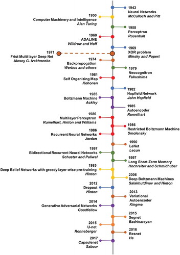
Figure 3. Illustration of convolutional neural architecture (CNN) architecture for classification of a radiological image for clinical diagnosis. (a) The CNN architecture shown here consists of two convolutional layers (each followed by a max-pooling layer), followed by two fully connected (dense) layers for image classification. (b) An example of a patch-based CNN applied to a multiparametric brain MRI dataset for segmentation of the different brain tissue types.
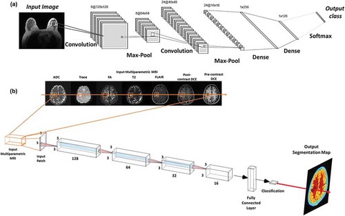
Figure 4. Illustration of an autoencoder used to learn a low dimensional representation of the high dimensional multiparametric MRI brain dataset by attempting to reconstruct it.
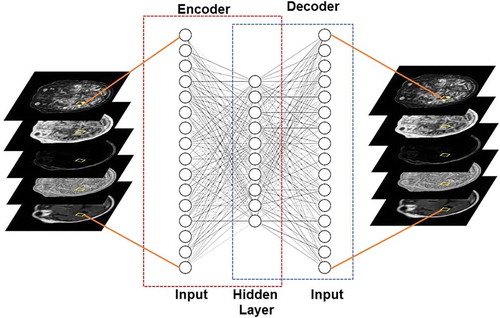
Figure 5. Illustration of a Deep Belief Network (DBN) with two hidden layers for segmentation of an example multiparametric MRI brain dataset. Each layer is pre-trained in an unsupervised fashion using Restricted Boltzmann Machines (RBMs) utilizing the outputs from the previous layer. The output from DBN segmentation on the example dataset is shown in the output layer.
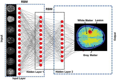
Figure 6. Illustration of the generative adversarial network (GAN) architecture. GANs consists of two neural network architectures competing against each other in a zero-sum game framework. One network generates candidates (generator) while the other evaluates them (discriminator). The goal of the generator is to synthesize realistic instances from the input data distribution while the goal of the discriminator is to differentiate between the true and synthesized instances of the input data distribution.
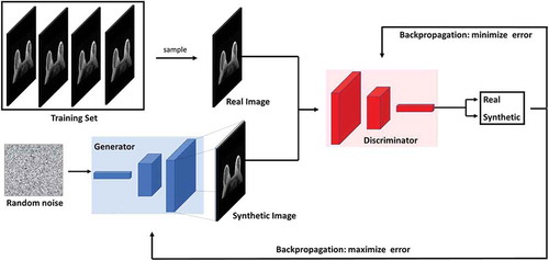
Figure 7. The timeline of important advancements in the field of texture and radiomics.
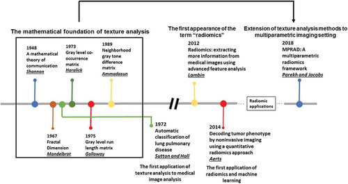
Figure 8. Illustration of the differences between GLCM radiomic features from conventional single image and multiparametric radiomics. (a). Single image radiomics features extract the inter-pixel relationships in-plane of a radiological image whereas, (b). the multiparametric radiomics extract the inter-tissue-signature relationships across multiple radiological images.
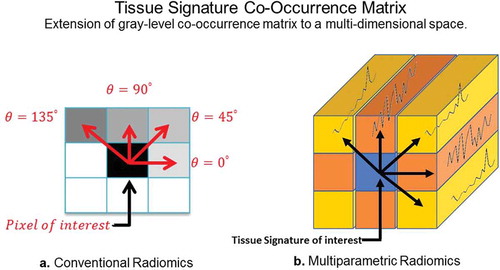
Figure 9. Illustration of multiparametric radiomic feature maps obtained from single and multiparametric radiomic analysis in a benign and malignant lesion. Top Row: Example of a patient with a benign lesion, where the straight yellow arrow highlights the lesion. There are clear differences between the single and multiparametric entropy radiomic images, where the multiparametric clearly demarcates the lesion. Bottom Row: Similar analysis on a patient with a malignant lesion (yellow arrow). Again, the multiparametric entropy map improves tissue delineation between the glandular and lesion tissue.
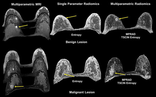
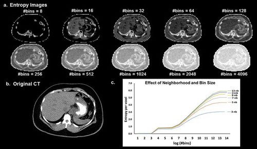
Figure 10. (a). Illustration of the dependence of the entropy value from the neighborhood size used for image filtering and image binning on a (b). CT image (Soft tissue window). (c). The curves of entropy vs bins appear to follow a distinct pattern where in the entropy values vary linearly with the log of number of bins within a certain range and remain more or less constant outside that range. The value of the entropy consistently increases with the increase in the size of the neighborhood filter.