The life cycle of a parthenogenetic population of Chara canescens from an interdunal Mediterranean pond

Figures & data

Figure 1. (A) The location and aerial photograph of the interdunal pond studied; taken by Matthieu Lasalle in 2015. (B) Basic features of water from the pond. TP: Total phosphorus; TN: Total nitrogen.

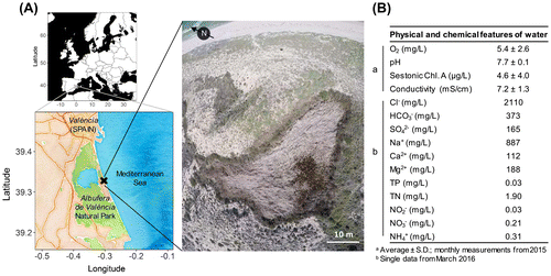
Figure 2. (A) The accumulated rainfall (bars) and the water level in the pond per month (line, mean ± SD when more than one value available). (B) The daily air temperature per month (black line, mean ± SD) at the surface of the pond, and the duration of the day (grey line) in Valencia, Spain. (C) The number of whorls of the main axis (black line) and the number of primary branches per shoot throughout the year (grey line) (mean ± SD by sampling date). (D) The reproductive effort per shoot (mean ± SD by sampling date), expressed as the number of fertile whorls per shoot (including lateral branches) divided by the number of whorls of the main axis. The higher values correspond to a higher proportion of fertile whorls per shoot, but also to a more lateral branching (presence of fertile multi-axis individuals). (E) The relative frequency of the shoots with each considered phenophase (non-swollen oogonia, swollen oogonia, ripe oospores) throughout the year, expressed as a percentage.

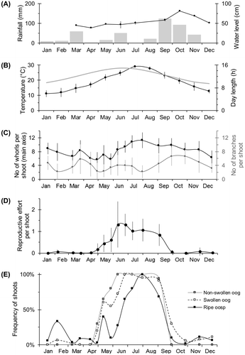
Figure 3. The life cycle of a parthenogenetic population of Chara canescens in the interdunal Mediterranean pond studied. The different events are distributed throughout the months of the year in a circular diagram. At the bottom, some boxplots show the distributions of the dimensions data measured for the fructifications (LPA: longest polar axis, including the coronula in oogonia; LED: largest equatorial diameter; ISI: isopolarity index; 0: non-swollen oogonia; 1: swollen oogonia; 2: ripe oospores).

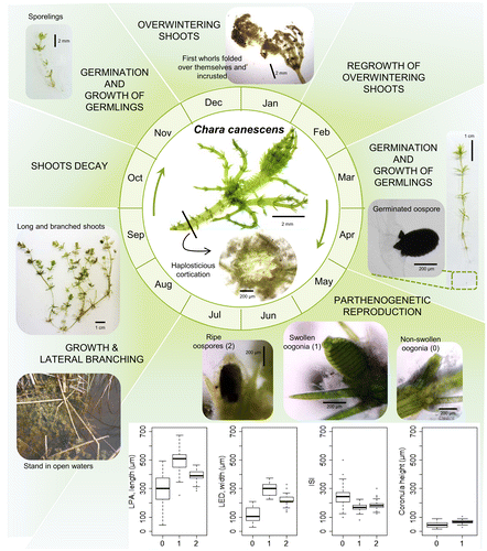
Figure 4. The distribution of the frequencies of all the measured oogonia and oospores in the different months of the year, according to their position within the shoot (number of whorl from the apex).

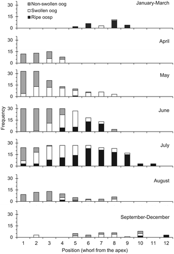
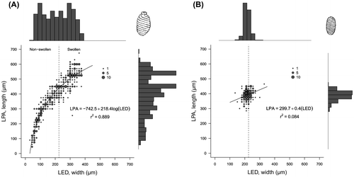
Figure 5. (A) The size relationship of the oogonia and (B) the oospores from the studied population of Chara canescens, including the respective logarithmic and linear relationships (p < 0.001) between their two main biometric characteristics (LED: largest equatorial diameter; LPA: longest polar axis). As the data are overlapping, the point size is proportional to the frequency of the oogonia/oospores in each case. The histograms of the frequencies for the two variables are also shown. The dashed lines show the LED value that was considered as the threshold for the swollen oogonia.

Table 1. The size ranges described in the literature for the swollen oogonia and the oospores from Chara canescens. LPA: longest polar axis, including the coronula in oogonia (marked with * if the coronula was excluded); LED: largest equatorial diameter; ISI: isopolarity index. 1: Groves and Bullock-Webster (1924); 2: Krause (1997); 3: Mann and Nambudiri (2005); 4: Cirujano et al. (2008); 5: Urbaniak and Gąbka (2015); 6: Calero and Rodrigo (this study).

	1	2	3	4	5	6
Swollen oogonia
LPA (μm)	600–750	550–800*	620–878	500–850*	550–750	255–675
LED (μm)	400–500	300–450	341–455	300–500	310–440	225–375
ISI	–	–	–	–	–	81–225
Coronula height (μm)	50–80	50–80	62 – 83	50–100	–	30–105
Convolutions	13–15	11–15	10–15	–	–	–
Ripe oospores
LPA (μm)	450–625	400–700	444–671	480–650	360–510	285–465
LED (μm)	275–400	200–400	258–341	210–350	205–295	135–330
ISI	–	–	–	–	–	125–300
Ridges	10–13	10–13	10–14	–	–	–

Groves, J., and G. R. Bullock-Webster. 1924. The British Charophyta, Volume II. Chareae. London: The Ray Society.

 Google Scholar

Krause, W. 1997. “Charales (Charophyceae).” In Sübwasserflora von Mitteleuropa [Pure Water Flora of Middle Europa], edited by H. Ettl, G. Gärtner, H. Heynig, and D. Mollenhauer, Vol. 18, 202. Stuttgart: Fischer.

 Google Scholar

Mann, H., and E. M. V. Nambudiri. 2005. “Charophytes of Insular Newfoundland II: Chara evoluta and Chara canescens.” The Canadian Field-Naturalist 119: 26–37.10.22621/cfn.v119i1.77

 Web of Science ®Google Scholar

Cirujano, S., J. Cambra, P. Sánchez Castillo, A. Meco, and N. Flor Arnau. 2008. Flora Ibérica. Algas Continentales. Carófitos (Characeae). [Flora Iberica. Continental Algae. Charophytes (Characeae)]. Madrid: Real Jardín Botánico, CSIC-Universidad de Barcelona.

 Google Scholar

Urbaniak, J., and M. Gąbka. 2015. Polish Charophytes. An Illustrated Guide to Identification. Wrocław: Wydawnictwo Uniwersytetu Przyrodniczego we Wrocławiu.

 Google Scholar