Satellite monitoring of chlorophyll-a threshold levels during an exceptional cyanobacterial bloom (2018-2019) in the Río de la Plata

Figures & data

Figure 1. a) Río de la Plata estuary, including its bathymetry, reference locations, main tributaries (Paraná and Uruguay rivers), and location of the study site in the northern coast; and b) study site and the measurement station (Latitude 34o45ʹ45.5” S and Longitude 56o32ʹ16.7”W) located in the Santa Lucía river mouth, approximately 40 km northwest of Montevideo (capital city of Uruguay).

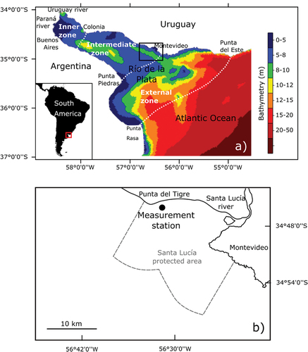
Figure 2. (a) ECO Triplet sensors integrated to the CTD prior to the deployment; (b-c) microscopic images of cyanobacteria-dominated samples collected at the measurement station: (b) Microcystis aeruginosa and (c) Dolichospermum sp.; (d) visual confirmation of cyanobacterial bloom during a field campaign in April, 2019.

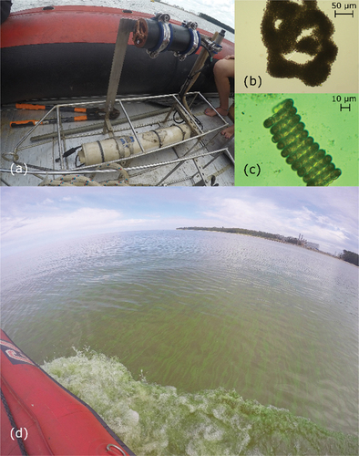
Figure 3. (a) Continuous records (every half an hour) of turbidity (left axis, brown line) and phycocyanin in vivo fluorescence (right axis, blue line) obtained at the measurement station; and (b) relative contribution of cyanobacteria to the total biomass at the measurement station. The solid (red) vertical lines included in panel (a) indicate Sentinel 2-MSI (S2) available images used to retrieve chl-a maps, while de dashed vertical lines indicate dates of the field campaigns (FC) where chlorophyll-a was extracted (see text).

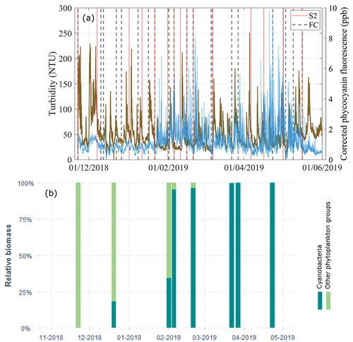
Figure 4. Daily discharge (in m³/s) for the main tributaries of the Río de la Plata, the Uruguay and Paraná rivers (left axis), including their combined flowrate (RdlP), and daily discharge of the local tributary, the Santa Lucía river (right axis), obtained from a rating curve approximately 50 km upstream of the river mouth (see text).

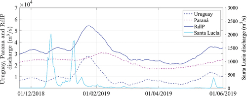
Figure 5. Distribution of wind velocities (in m/s) for the study region in the period November 2018-May 2019, obtained from reanalysis data (see text). Each data point indicates the magnitude and direction from which the wind is coming. Warmer (colder) colors represent more (less) density of data points. The 10^th, 50^th and 90^th percentiles (P10, P50 and P90, respectively) are included for each of the 16 discrete directions.

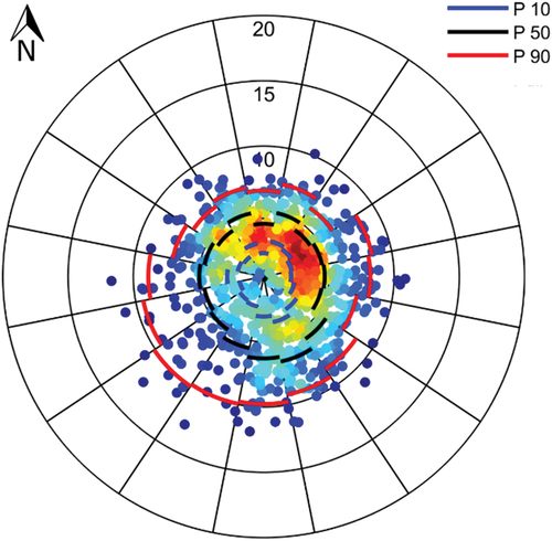
Figure 6. Time series of continuous measurements (half an hour) of water temperature (left axis) and salinity (right axis) at the measurement station.

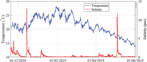
Figure 7. Sequence of Sentinel 2 images between late November 2018 and mid-January 2019. Left panels: RGB composites, with the land indicated in black. Central panels: the chl-a threshold of 10 µg/L as detected by none (gray), only one (red) or both (black) of the chl-a indices described in Section 3. Right panels: threshold maps for chl-a levels above 10 and 24 µg/L, simultaneously detected by both chl-a indices. In central and right panels, the land is indicated in white. The timeline also includes: extracted chl-a concentrations when available, peaks in the Uruguay, Paraná, Río de la Plata and Santa Lucía river discharges (QU, QP, QRdlP, and QSL, respectively), and relevant local wind events.

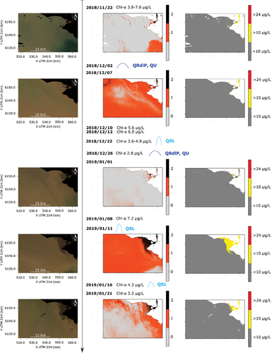
Figure 8. Same as Figure 7 but from late January to late February, 2019.

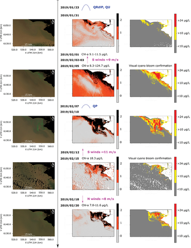
Figure 9. Same as Figure 7 but from March to mid-May, 2019.

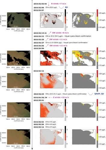
Figure 10. Causal loop diagram, based on the one presented in [52], but for cyanobacterial accumulation at the study site. Positive (+) feedbacks are indicated with continuous (green) arrows; Negative (-) feedbacks are shown with dashed (red) arrows; and dash-dotted (blue) arrows represent either positive or negative (+/-) feedbacks according to the characteristics of the driver (e.g. wind direction).

Nagy GJ, Muñoz N, Verocai JE, et al. Integrating Climate Science, Monitoring, and Management in the Rio de la Plata Estuarine Front (Uruguay). In: Leal Filho W, Alves F, Caeiro S, et al., editors. International Perspectives on Climate Change Climate Change Management. Switzerland: Springer; 2014. p. 79–92.

 Google Scholar