A Computational Framework for Preserving Privacy and Maintaining Utility of Geographically Aggregated Data: A Stochastic Spatial Optimization Approach

Figures & data

Figure 1 Data involved in the disclosure problem. (A) Hypothetical individual-level data from twenty-four people in three census blocks. Each individual has two attributes, marital status and age group. (B) Three data sets aggregated from the individual-level data in (A). (C) Auxiliary data that contain personal identifiers.

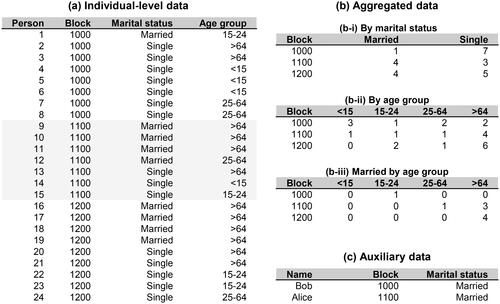
Figure 2 Matrix representation of the individual-level data. Specifically, a 7 × 3 matrix X is used to represent the individual-level data in Figure 1A.

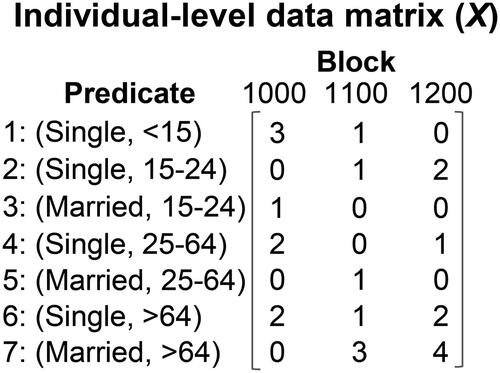
Figure 3 Aggregation using a query matrix. (A) A 2 × 7 query matrix A consisting of two counting queries, which are used to obtain population counts by marital status in each block. (B) A 2 × 3 matrix Y that represents the aggregated data in Figure 1Bi, which is obtained by multiplying the query matrix A with the individual-level data matrix X in Figure 2B.

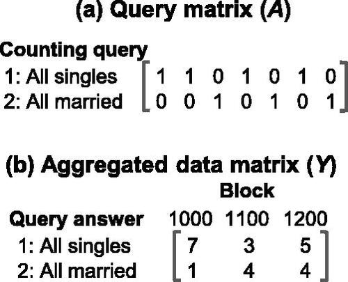
Figure 4 Schematic diagrams of transition probabilities. For our example in Figure 2, consider two one-elements in block 1100: (A) person 14 who is the only individual satisfying predicate (Single, < 15), and (B) person 13 who satisfies predicate (Single, > 64). These two individuals need to be protected and assigned to candidate blocks because they have a high disclosure risk of one. Three possible assignments can be made for each individual, as illustrated by the three arrows in each diagram. We use transition probabilities to describe the likelihood of each assignment.

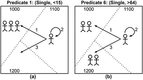
Figure 5 A flowchart of the computational framework.

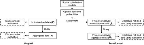
Table 1. Worst-case disclosure risks

			Worst-case disclosure risks
County	Data type	Data	Global disclosure risk (${\tau }^{*}$)	Population uniqueness rate (${\varphi }^{*}$)
Franklin	Individual-level	VER	0.167	0.086
	Aggregated	ER	0.157	0.081
	Aggregated	R	0.094	0.042
Guernsey	Individual-level	VER	0.215	0.114
	Aggregated	ER	0.187	0.086
	Aggregated	R	0.141	0.057

Table 2. User-specified parameters and their values

Input	Description	Value range
rj	Capacity of candidate locations	10
wkij	Error of assigning one individual	Penalty value set to 50
tijk	Coverage of candidate locations	Determined by two coverage principles: free assignment and spatial proximity
λ	Integer to determine λ-elements	1, 2, 3
N	Number of elements in the individual-level data matrix	7,952
u	Error budget	0.05 N, 0.1 N, 0.5 N, N, 1.5 N, 2 N

Figure 6 Global disclosure risks (τ) of data transformed using the minimum error model for (A) Franklin County and (B) Guernsey County.

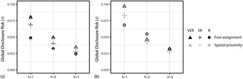
Figure 7 Global disclosure risks (τ) of data transformed using results from the maximum protection model for (A) Franklin County and (B) Guernsey County.

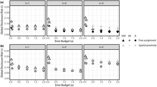
Figure 8 Population uniqueness rates ($\varphi$) of data transformed using the maximum protection model for (A) Franklin County and (B) Guernsey County.

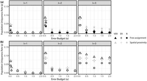
Table 3. Minimum penalized error required to assign all at-risk individuals

		Minimum penalized error
County	Λ	Free assignment	Spatial proximity
Franklin	1	0.095 N	0.526N
	2	0.171 N	1.997N
	3	1.400 N	4.531N
Guernsey	1	1.187 N	1.187N
	2	2.905 N	2.905N
	3	13.317 N	13.317N

Figure 9 Symmetric mean error (SME) of data transformed using results from the minimum error model for (A) Franklin County and (B) Guernsey County.

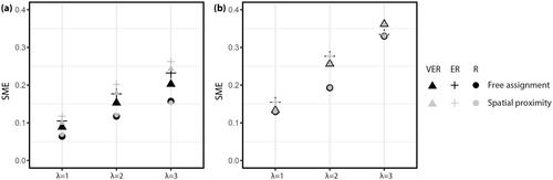
Figure 10 Symmetric mean error (SME) of data transformed using results from the maximum protection model for (A) Franklin County and (B) Guernsey County.

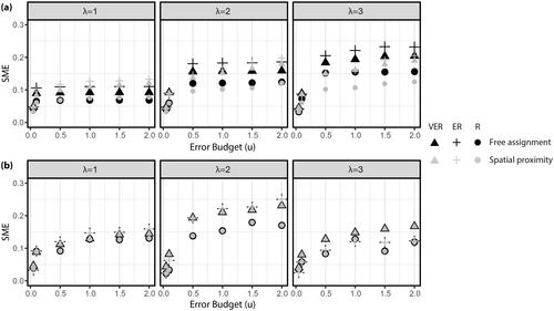
Figure 11 Impacts of two coverage principles on local indicators of spatial association (LISA) patterns for the percentage of non-Hispanic American Indian and Alaska Native (AIAN) population. The percentage of non-Hispanic AIAN population is derived from (A) the original aggregated data ER, as well as (B) and (C) two transformed ER using the minimum error model with λ = 3 under two coverage principles. Note: HH = statistically significant clusters of high values; LL = clusters of low values; HL = outliers with high values surrounded primarily by low values; LH = outliers with low values surrounded primarily by high values.

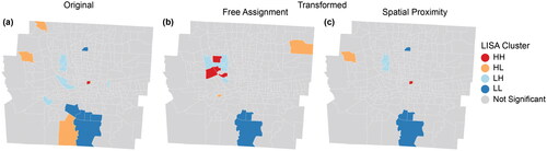
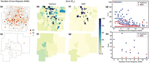
Figure 12 Error introduced by the differential privacy-based TopDown algorithm and the minimum error model (MEM) at the census tract level. (A) and (E) Original count of non-Hispanic American Indian and Alaska Natives (AIANs) in each census tract of Franklin and Guernsey Counties, respectively. (B) and (C) Error for Franklin County. (F) and (G) Error for Guernsey County. (D) and (H) Relationship between the count and the error introduced by the two methods for Franklin and Guernsey Counties, respectively. Each symbol represents a census tract.

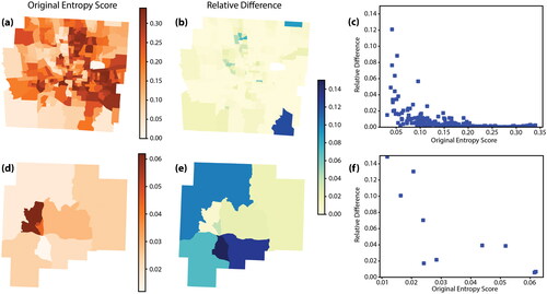
Figure 13 Effects of relocating individuals on demographic diversity. (A) and (D) Entropy score calculated using the original ER in Franklin and Guernsey Counties, respectively. (B) and (E) Relative difference between entropy scores of the original and transformed ERs in Franklin and Guernsey Counties, respectively. (C) and (F) Relationship between the original entropy score and the relative difference in Franklin and Guernsey Counties, respectively.