Figures & data
Figure 1. Chart of the automatic algorithm to compute the segmentation of the most anterior lateral and medial points, along with the deepest point of the trochlear groove.
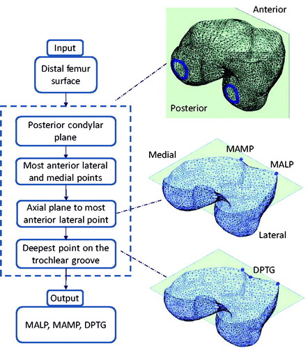
Figure 2. Posterior and distal intercoldylar notch points on the internal trochlear region (a). The ventral aspect of the trochlear surface segmented on the distal femur surface (b).
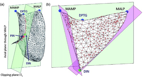
Figure 3. Lateral and medial sides of the trochlear surface (a). HP modeling of the overall trochlear surface (b). Medial HP modeling (c). Lateral HP modeling (d). Medial and lateral HPs share the location, the orientation and the bL factor.
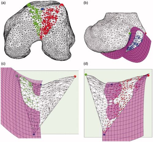
Table 1. Variations of the estimated global HP parameters as a function of the isotropic scaling applied to the sample trochlear surface of the sample patients.
Figure 4. Box plots of the aG and bG distributions for the two subgroups, dysplastic and normal. Median and lower–upper percentiles are displayed.
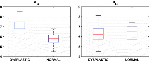
Figure 5. aG versus bG graph along with sample distal femur surfaces. Blue dots indicate patients diagnosed with no dysplasia.
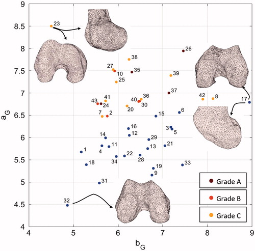
Figure 6. Five distal femur surfaces along with their corresponding aG parameters. A monotonic increase of the parameter corresponds to a decrease of the roundness of the trochlea.
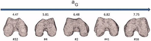
Figure 7. Box plots of the aG distributions of the three dysplastic subgroups (left panel).
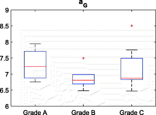
Figure 8. Box plots of the aLl and aLm distributions for the two subgroups, dysplastic and normal. Median and lower–upper percentiles are displayed.
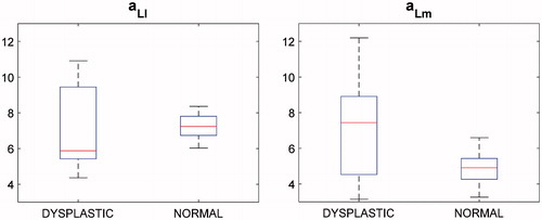
Figure 9. aLm versus aLl graph along with sample distal femur surfaces. Blue dots indicate patients diagnosed with no dysplasia.
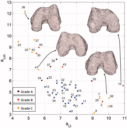
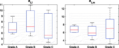
Figure 10. Box plots of the aLl and aLm distributions of the three dysplastic subgroups.