The brain MRI image sparse representation based on the gradient information and the non-symmetry and anti-packing model

Figures & data

Figure 1. The brain MRI images.

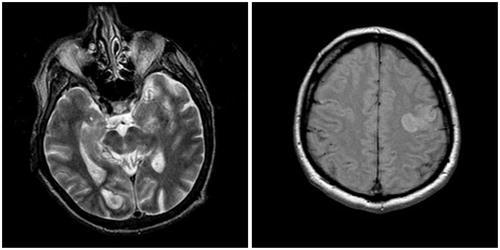
Figure 2. The partition results by using the NAM. (a) NAM based on the gray information, (b) NAM based on the gradient information.

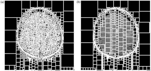
Figure 3. Four test images used in our experiments.

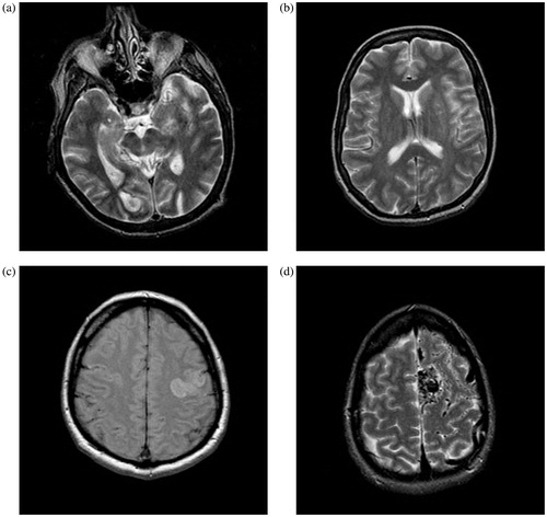
Figure 4. Nonlinear approximation by using different methods. In the first line and third line, the image Figure 3(a) is reconstructed from 500-most significant coefficients, and the corresponding error images are presented in the second line and forth line. Brighter pixel represents larger error in error images.

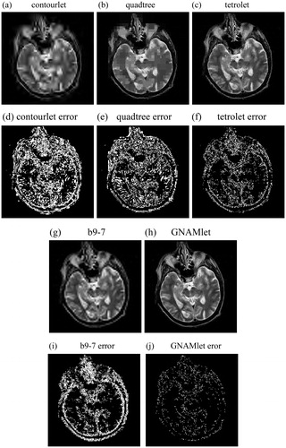
Figure 5. Nonlinear approximation by using different methods. In the first line and third line, the image Figure 3(c) is reconstructed from 1250-most significant coefficients, and the corresponding error images are presented in the second line and forth line. Brighter pixel represents larger error in error images.

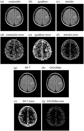
Table 1. The PSNR values obtained by different methods with η = 500, η = 1250 and η = 2500 respectively.

Method	η	Figure 3(a)	Figure 3(b)	Figure 3(c)	Figure 3(d)
contourlet	500	22.35	34.35	26.74	25.95
	1250	24.93	27.43	30.26	28.70
	2500	27.19	29.87	32.94	31.17
quadtree	–	25.08	27.25	27.38	24.86
tetrolet	500	26.95	28.99	30.26	30.20
	1250	28.73	31.36	32.90	32.27
	2500	30.84	33.94	35.85	34.75
b9-7	500	23.99	24.55	27.86	27.20
	1250	24.02	24.55	27.86	28.38
	2500	27.10	30.15	34.03	32.73
GNAMlet	500	31.27	34.40	34.20	33.36
	1250	32.77	36.29	36.75	35.05
	2500	34.72	38.58	39.76	37.43

Table 2. Comparison of different transforms regarding computation time (in second).

Method	Decomposition time	Reconstruction time
b9-7	0.02	0.009
Tetrolet	0.29	0.210
Contourlet	0.61	0.047
Quadtree	3.72	0.012
GNAMlet	3.51	0.330