Three-dimensional analysis of acetabular orientation using a semi-automated algorithm

Figures & data

Figure 1. Three-dimensional pelvic coordinate system. The most ventral points were automatically located on the anterior superior iliac spine and pubic tubercles bilaterally (red points) and were used to establish the three-dimensional pelvic reference frame. The anterior pelvic plane, or coronal plane (red plane), consisted of the anterior superior iliac spine and the pubic tubercle points bilaterally. The sagittal plane (green plane) contained the line (dashed line) connecting the two midpoints of the bilateral anatomical landmarks and was normal to the APP. The axial plane (blue plane) was normal to both coronal and sagittal planes.

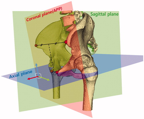
Figure 2. An algorithm for determining the acetabular rim plane, which consisted of six steps. Step 1: Specifying the ROI for each femoral head (Red box). Step 2: Identifying a best-fit sphere (blue) using planar circles (red) detected by SHT. Step 3: Reconstructing each slice using the scan line. The yellow points detected by the corner detection algorithm were candidates for the acetabular rim points. Step 4: Generating the pseudo plane and acetabular coordinate system. The blue points were selected by a RANSAC algorithm; the red points were determined as outliers. The pseudo plane (dashed line) was determined by blue points, and the plane (solid line) was obtained by moving the pseudo plane 1 cm in the direction of -ZA. Step 5: Determining the true acetabular rim points. The true rim point was defined by a virtual ray. The direction of the virtual ray was adjusted by changing the azimuth (θ) and angle (φ). The first-hit voxels were defined as the true rim points. Step 6: The plane fitting the acetabular rim points (yellow) determined the true acetabular rim plane (white).

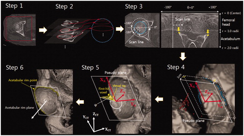
Table 1. Elapsed time of the algorithm for two phase including manual operation (n = 20).

Measure	Phase 1^†	Phase 2^‡	Overall process
Mean (sec)	89.04	128.88	217.80
SD* (sec)	23.79	9.19	28.08
Range (sec)	61–141	116–149	181–280

* Standard deviation.

† Pelvic coordinate system determination.

‡ Acetabular rim plane determination.

Table 2. ICC values for calculation of the angles on two separate occasions (n = 20).

Measure	Left inclination	Left anteversion	Right inclination	Right anteversion
Trial 1 vs. Trial 2*	0.975	0.988	0.985	0.976
Rater 1 vs. Rater 2^†	0.945	0.976	0.954	0.964
Original volume vs. Rotated volume^‡	0.960	0.967	0.975	0.956

* Intra-observer reliability. The values for each method were calculated for two trials at least 4 weeks apart.

^† Inter-observer reliability. The values for each method were calculated for two raters.

^‡ The rotation angle range on the arbitrary axis was 15°–30°.

Values are ICC scores with 95% confidence intervals (Cronbach alpha values of 0.90–1.00 are considered almost perfect).

Table 3. Acetabular inclination and anteversion by age and gender (n = 200).

Group		# of patients	Inclination angle			Anteversion angle
			Mean	SD*	Range	Mean	SD*	Range
Age <70 years	Males	34	50.64	4.43	37–62	16.07	3.79	4–23
	Females	60	50.11	4.09	39–60	15.48	3.89	9–23
Age ≥70 years	Males	26	51.04	3.96	40–59	16.16	4.28	6–24
	Females	80	50.02	4.43	40–62	16.05	4.23	4–23
All patients		200	50.03	4.22	37–62	15.84	4.02	4–24

* SD = standard deviation.

Figure 3. Acetabular inclination by age and sex. Regression analysis indicated no evidence of an association.

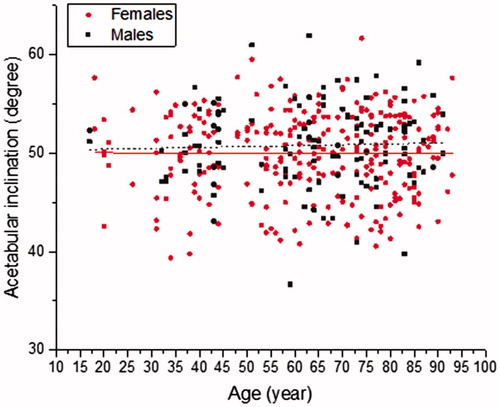
Figure 4. Acetabular anteversion by age and sex. Regression analysis indicated no evidence of an association.

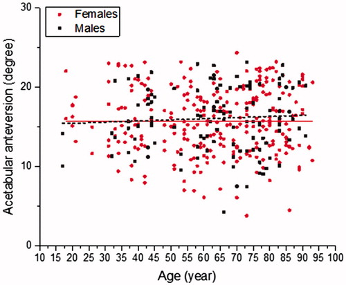
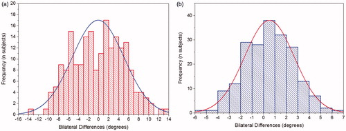
Figure 5. Frequency and magnitude of intra-patient bilateral differences (left minus right). Relative symmetry was shown for (a) anatomic anteversion and (b) anatomic inclination.