
Figures & data
Figure 1. Nominal cut surfaces for a femur are shown in coronal (A) and sagittal (B) views. The names of the five femoral cut planes are also shown. The laser scanned cut surfaces of the same femur are also shown in coronal (C) and sagittal (D) views.
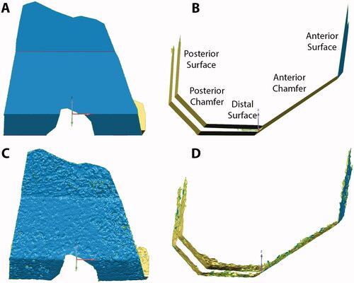
Figure 2. Femoral cut surfaces were selected (red) based on crease angles of 15° (A), 20° (B), and 25° (C). As the crease angle is increased, more porous regions are selected.
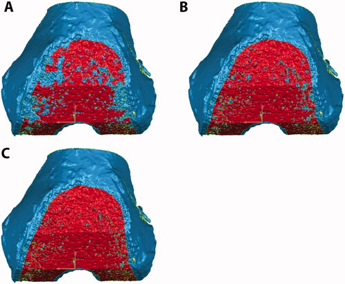
Figure 3. Micro-CT (A), gross photography (B), and laser scan (C) show the same femoral anterior chamfer cut surface for one representative specimen. Dark regions in the micro-CT are porous regions that are not densely occupied by trabeculae. An appropriate crease angle was used to select the cut bone surface (red) in the laser scan without significant trabecular porosity.
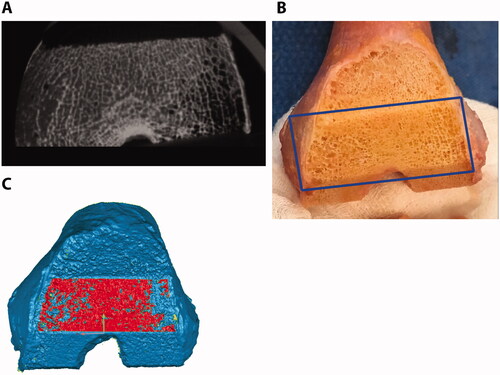
Figure 4. Deviation maps show the distance between each cut surface and the best-fit plane. The best-fit plane was created without including the boundaries of the surface to avoid regions where the surgeon manually removed marginal bone. Flatness was computed as the standard deviation of the distance between the cut surface and the best-fit plane. Scale is in mm.
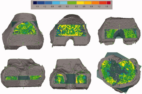
Figure 5. Steps for computing femoral cut plane angular errors. Planes were best-fit to each cut surface. The angle between each cut plane and all other cut planes, even non-adjacent ones, was calculated for a total of twenty angular differences for each femur. The figure shows the four angles that were calculated for the anterior chamfer (A) and distal surface (B). Similar measurements were made for the other three surfaces. The twenty angle errors were computed by subtracting the nominal angles from the measured angles. This measurement was not performed for the tibia given it only has one planar cut.
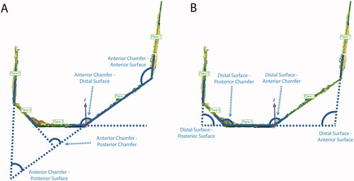
Figure 6. Steps for computing distance errors for the femoral cuts from the nominal cut planes. All five cut surfaces were shape matched to the nominal cut planes. A 3D deviation map was then computed to determine which percentage of the cut surface was within the tolerance of ±1 mm. Green colors indicate that the surface was within tolerance, while red and blue colors indicate that the actual cut was too far outside and inside the planned cut, respectively.
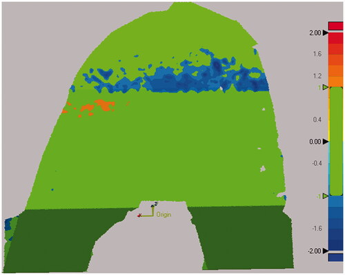
Figure 7. Microradiographs of a sagittal section of the femur (A) and coronal section of the tibia (B), show the flatness of each cut. Arrows point to portions of bone that were uncut as a result of the chosen preoperative plan and would be outside of where the implant would rest and were not analyzed. To create the microradiographs, the bones were fixed in 10% Neutral Buffered Formalin, dehydrated in ascending grades of ethanol, infiltrated, and embedded in polymethyl methacrylate. Once the specimens were polymerized, 2 mm thick sections were made from each polymerized block. High-resolution contact radiographs were then made of each section.
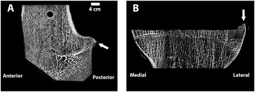
Figure 8. SEM images of a tibia without an implant (A) and a different tibia with cemented implant (B), with Gray = Bone, White = Implant, and Black = Soft Tissue/Cement. The cut surface is noticeably flattered on the specimen that has an implant. Comparison of a smooth vs. frayed trabecula (C) from SEM image. For the femur with an implant, the ratio of smooth vs. frayed trabecular was similar to the femur without an implant (67 vs. 68% smooth trabeculae), but for the tibia, the one with an implant had a higher amount of smooth trabeculae (37 vs. 47%). To create the SEM images, one section from each specimen was ground and polished to an optical finish. The polished ∼2 mm-thick sections were coated with a thin conductive layer of carbon for ∼25 s and imaged using a JEOL JSM-6610 SEM equipped with a backscatter electron (BSE) detector and associated imaging software. Digital BSE images were captured along the entire resected surface and then stitched together for (A) and (B).
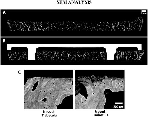
Table 1. Flatness errors (mean ± standard deviation, range) for the femoral and tibial cut surfaces (mm).
Table 2. Angular errors (mean ± standard deviation) for both the femoral cuts and implants (degrees).
Table 3. Percentage of the femoral cut surfaces that would have a <1 mm bone-implant gap.