Performance assessment of surgical tracking systems based on statistical process control and longitudinal QA

Figures & data

Figure 1. Testbed for tracker QA. (a) Setup for an EM tracking system (Aurora #1), showing the field generator, phantom with reference marker, pointer, and software interface. (b) Setup for an IR tracking system (Vicra #1). (c) software interface showing coronal, axial, sagittal, and surface-rendered views of the phantom with fiducial points (yellow) overlaid after tracker-to-image registration. Also shown are the software controls and outputs of QA measurements.

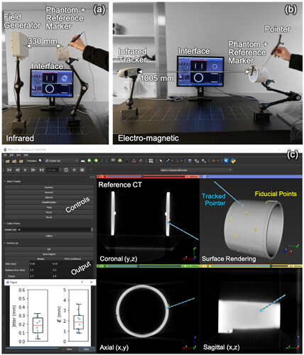
Table 1. Summary of test outcomes associated with QA measurement results relative to established control limits.

Test result	Outcome
0 tests above UCL or below LCL	Pass
1 test above UCL	Note to operator
1 or more tests below LCL	Note to operator
2 tests above UCL in same metric category (i.e. Jitter or $\epsilon$)	Alert to operator
2 or more tests above UCL in different metric categories (i.e. Jitter and $\epsilon$)	Failure

Figure 2. Range in TRE according to the model of Equation (1)(1) $$〈{\mathrm{TRE}\left(x\right)}^2〉=\frac{1}{N_r}(1+\frac{1}{3}\sum _{k=1}^3\frac{d_k^2}{f_k^2})〈{\mathrm{FLE}}^2〉$$(1) over all target positions in LOO analysis for all configurations of $N$ point positions ($N_r=N-1$ registration fiducials and 1 target position). Cases $N$ = 4, 7, and 10 are shown, the last giving a narrow range suggesting that all measurements are representative of a similar underlying statistical distribution in TRE. Violin plots show the range (upper and lower horizontal lines), distribution of samples (shaded envelope), and median (horizontal line). The vertical arrow signifies samples in the upper tail of the distribution.

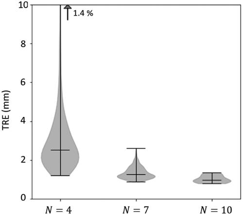
Figure 3. Spatial distribution in TRE computed by Equation (1)(1) $$〈{\mathrm{TRE}\left(x\right)}^2〉=\frac{1}{N_r}(1+\frac{1}{3}\sum _{k=1}^3\frac{d_k^2}{f_k^2})〈{\mathrm{FLE}}^2〉$$(1) over a cross section of the phantom for $N$ = 4, 7, and 10 registration fiducials for Inferior/Superior fiducial configurations. Registration fiducial/target locations (magenta/green) are projected onto the cross section. The low TRE magnitude, high degree of spatial uniformity, and similarity in TRE distributions for the $N$ = 10 case supports LOO analysis as a means to obtain 10 TRE estimates in a single QA test with 10 measurement points.

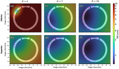
Figure 4. Measurements of error $\epsilon$ (from Phase I definition of control limits) as a function of the number of point positions for a single example Superior (gray) and Inferior (black) fiducial configuration. (a) Electromagnetic tracker (Aurora #2). (b) infrared tracker (Vicra #2). theoretical model fits are shown as dashed lines.

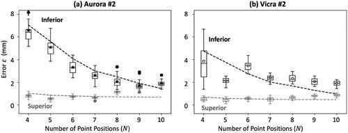
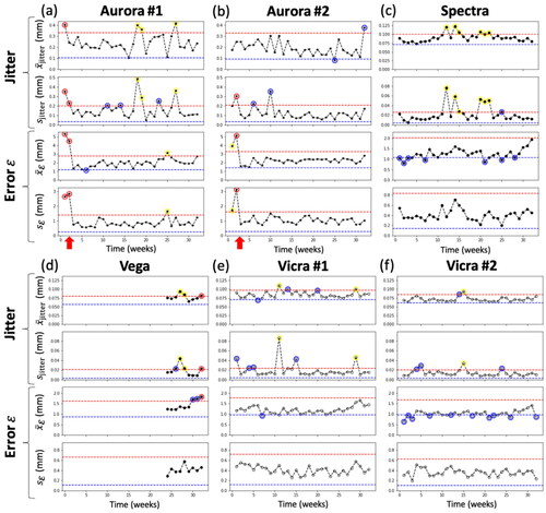
Figure 5. Control limits in Jitter (top row) and error $\epsilon$ (bottom row) for the six tracking systems. Data points rejected from the analysis are marked with a red circle, leaving at least 25 measurements for the establishment of upper and lower control limits.

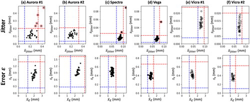
Table 2. Upper and lower control limits for the mean and standard deviation in Jitter and error $\epsilon$ for each tracking system.

Tracker	Metric	LCL (mm)	UCL (mm)
Aurora #1	${\overline{x}}_{\mathrm{jitter}}$	0.11	0.33
	$s_{\mathrm{jitter}}$	0.03	0.20
	${\overline{x}}_{\epsilon }$	1.21	2.79
	$s_{\epsilon }$	0.23	1.39
Aurora #2	${\overline{x}}_{\mathrm{jitter}}$	0.09	0.33
	$s_{\mathrm{jitter}}$	0.04	0.21
	${\overline{x}}_{\epsilon }$	1.44	3.28
	$s_{\epsilon }$	0.27	1.62
Spectra	${\overline{x}}_{\mathrm{jitter}}$	0.07	0.10
	$s_{\mathrm{jitter}}$	0.004	0.03
	${\overline{x}}_{\epsilon }$	1.08	2.02
	$s_{\epsilon }$	0.14	0.83
Vega	${\overline{x}}_{\mathrm{jitter}}$	0.06	0.08
	$s_{\mathrm{jitter}}$	0.003	0.02
	${\overline{x}}_{\epsilon }$	0.87	1.62
	$s_{\epsilon }$	0.11	0.66
Vicra #1	${\overline{x}}_{\mathrm{jitter}}$	0.07	0.10
	$s_{\mathrm{jitter}}$	0.004	0.02
	${\overline{x}}_{\epsilon }$	0.96	1.77
	$s_{\epsilon }$	0.12	0.71
Vicra #2	${\overline{x}}_{\mathrm{jitter}}$	0.06	0.08
	$s_{\mathrm{jitter}}$	0.003	0.02
	${\overline{x}}_{\epsilon }$	0.96	1.67
	$s_{\epsilon }$	0.10	0.63

Figure 6. Phase II longitudinal QA tests for each tracking system. UCL and LCL are marked by red and blue dashed lines, respectively. Interventions are marked by red arrows. Consistent with Table 1, Notes are marked by blue circles, Alerts are marked by yellow circles, and Failures are marked by red circles.