Figures & data
Figure 1. Boxplots of 1000 simulated values of in-control (γ = 1) CARL. Parameter values are m = 50, n = 5, α = 0.005, ϵ = 0.1, and p = 0.1. The dashed vertical line indicates CARLtol = 1/αtol = 182, and the p-quantiles are indicated with an added vertical line in the boxplots.
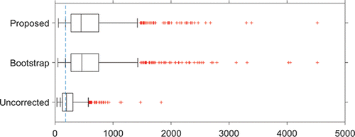
Figure 2. Boxplots of 1000 simulated values of out-of-control (γ = 1.5) CARL. Parameter values are m = 50, n = 5, α = 0.005, ϵ = 0.1 , and p = 0.1.
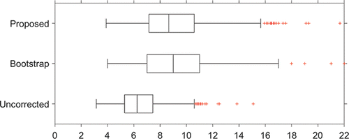
Figure 3. Boxplots of 1000 simulated values of in-control (γ = 1) CARL. Parameter values are m = 50, n = 5, α = 0.005, ϵ = 0, and p = 0.05. The dashed vertical line indicates CARLtol = 1/αtol = 200, and the p-quantiles are indicated with an added vertical line in the boxplots.
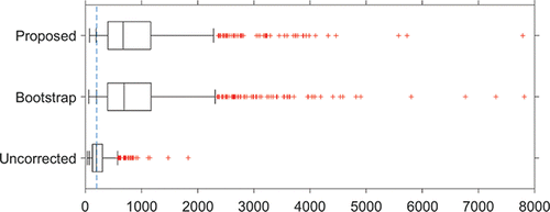
Figure 4. Boxplots of 1000 simulated values of out-of-control (γ = 1.5) CARL. Parameter values are m = 50, n = 5, α = 0.005, ϵ = 0 , and p = 0.05.
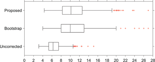
Table 1. Required values of a and b (and a0 and b0) for different estimators used in the calculation of the adjusted control limit.
Table 2. Control limit coefficients: Unadjusted and adjusted for Sp with ϵ = 0.10 (α = 0.005). Every second row (in italics) gives the ratio between the adjusted and the unadjusted limit.
Table 3. Control limit coefficients: Unadjusted and adjusted for Sp with ϵ = 0.20 (α = 0.005). Every second row (in italics) gives the ratio between the adjusted and the unadjusted limit.
Table 4. Out-of-control CARL for γ = 1.5 of the S chart with and without the adjusted limits, when W = 1 (α = 0.005).
Table 5. Out–of-control CARL for γ = 2.0 of the S chart without and with adjusted limits, when W = 1 (α = 0.005).
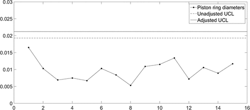
Figure 5. Application of the proposed control chart to the piston ring data set. Both the unadjusted and adjusted control limits are indicated.
