Impact Assessment of Traffic Noise in a Densely Populated Industrial City, Faisalabad Pakistan Using Geostatistical Approach and Development of Sustainable Transportation System Framework

Figures & data

Figure 1. Study areaE, map of Faisalabad city.

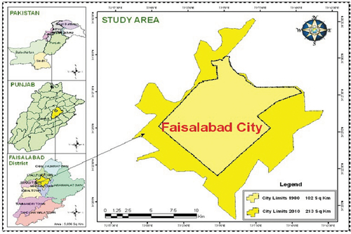
Figure 2. Sampling sites of Faisalabad city.

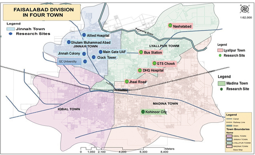
Table 1. Statistical analysis of average noise levels at 12 sites.

Timing	Lavg(min)	Lavg(max)	Lavg(mean)	SD	Kurtosis	Skewness
8:00–9:00 am	87	97.8	94.2	3.01	2.68	0.018
1:00–2:00 pm	87.0	99.8	93.4	3.016	2.68	0.018
7:00–8:00 pm	88.3	101.6	94.7	3.300	3.40	0.149

Table 2. Cross-validation of L_avg (characteristic parameters of variogram models).

Average sound level Lavg	Mean Error	Root Mean Square Error	Average Standard Error		Mean Standardized Error	Root Mean Square Standardized Error	Best fit model
8:00–9:00 am	0.8812	6.513	7.496	0.09495		0.8612	Gaussian
1:00–2:00 pm	0.2664	4.216	4.724	0.04386		0.8914	Gaussian
7:00–8:00 pm	0.244	3.943	4.088	0.05568		0.9722	Spherical

Table 3. Statistical analysis of peak noise levels at 12 sampling sites.

Timing	Lpeak(min)	Lpeak(max)	Lpeak(mean)	SD	Kurtosis	Skewness
8:00–9:00 am	88.9	113.9	98.4	5.452	3.07	0.826
1:00–2:00 pm	95.1	108.9	102.9	3.637	3.23	−0.709
7:00–8:00 pm	91.7	108.8	104.1	2.699	3.14	−0.439

Table 4. Cross-validation of L_peak (characteristic parameters of variogram models).

Average sound level Lpeak	Mean Error	Root Mean Square Error	Average Standard Error	Mean Standardized Error	Root Mean Square Standardized Error	Best Fit Model
8:00–9:00am	1.723	8.58	11.06	0.1288	0.825	Gaussian
1:00–2:00 pm	0.2894	5.108	5.947	0.03317	0.8669	Gaussian
7:00–8:00 pm	−0.0483	5.401	5.863	−0.008287	0.9221	Spherical

Figure 3. Histogram of average noise level data.

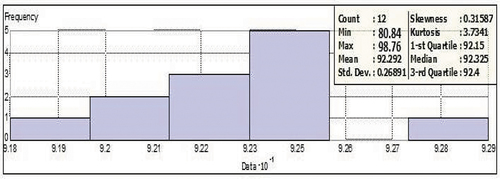
Figure 4. Normal Q-Q plot of average noise level data.

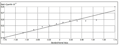
Figure 5. Gaussian model for average noise level data (8.00–9.00 AM).

Figure 6. GIS map of average sound level data (8–9 am).

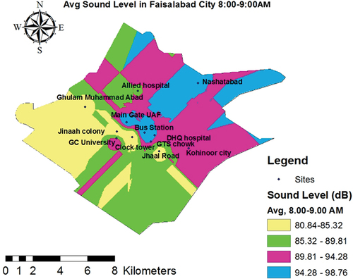
Figure 7. Histogram of average noise level data.

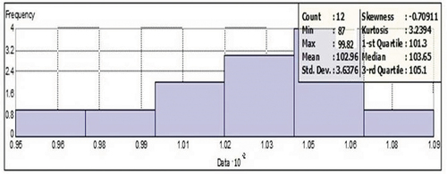
Figure 8. Normal Q-Q plot of average noise level data.

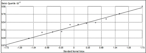
Figure 9. Gaussian model for average noise level data (1.00–2.00 PM).

Figure 10. GIS map of average sound level data (1–2 pm).

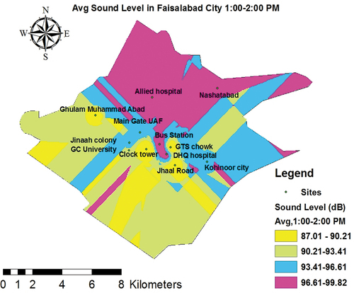
Figure 11. Histogram of average noise level data.

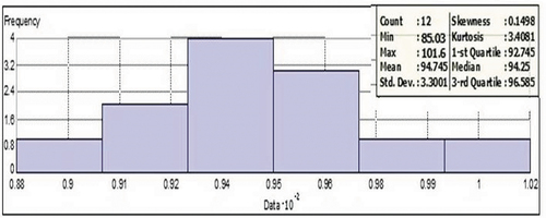
Figure 12. Normal Q-Q plot of average noise level data.

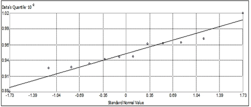
Figure 13. Spherical model for average noise level data (7.00–8.00 AM).

Figure 14. GIS map of average sound level data (7–8 pm).

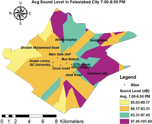
Figure 15. Histogram of peak noise level data.

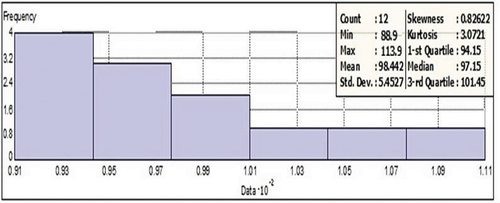
Figure 16. Normal Q-Q plot of peak noise level data.

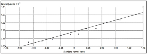
Figure 17. Gaussian model for peak noise level data (8.00–9.00 AM).

Figure 18. GIS map of peak sound level data (8–9 am).

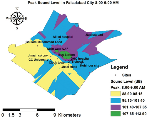
Figure 19. Histogram of peak noise level data.

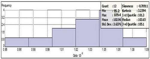
Figure 20. Normal Q-Q plot of peak noise level data.

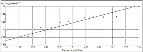
Figure 21. Gaussian model for peak noise level data (1.00–2.00 PM).

Figure 22. GIS map of peak sound level data (1–2 pm).

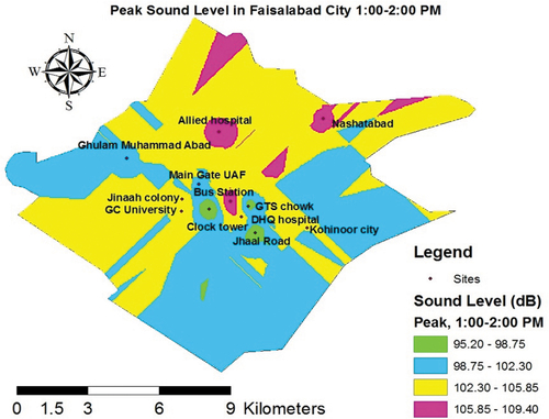
Figure 23. Histogram of peak noise level data.

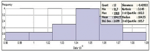
Figure 24. Normal Q-Q plot of peak noise level data.

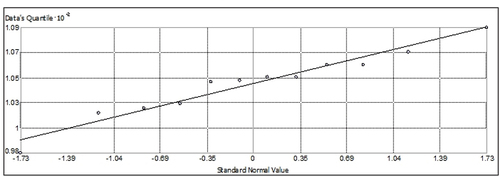
Figure 25. Spherical model for peak noise level data (7.00–8.00 PM).

Figure 26. GIS map of peak sound level data (7–8 pm).

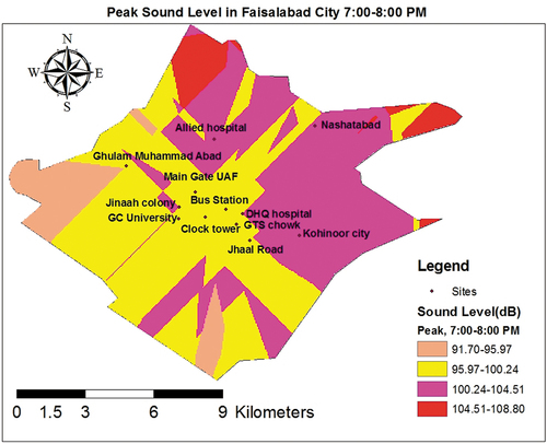
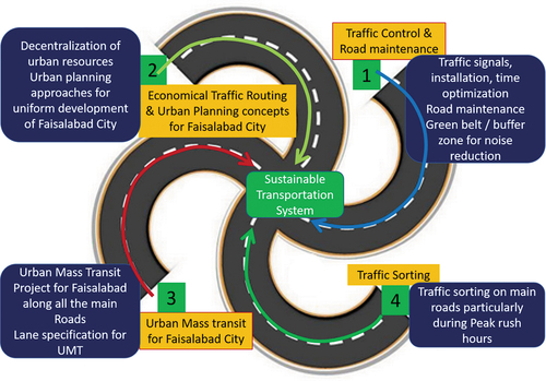
Figure 27. Four roads to a sustainable transportation system in Faisalabad city.