Figures & data
Figure 1. Geographical setting of the Ligurian Sea, with its position within the Mediterranean (inset). Localities cited in the text are indicated.
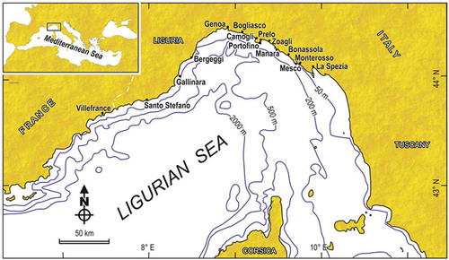
Figure 2. Multidecadal (1980–2018) trends of yearly averages of temperatures in Liguria. (a) Air temperature, measured at the meteorological observatory of Genoa university. (b) Sea surface temperature (SST), from NOAA satellite data (www.esrl.noaa.gov/psd/cgi-bin/data/timeseries/timeseries1.pl). In both graphs, the smoothed thick lines depict the 6th degree polynomial fit.
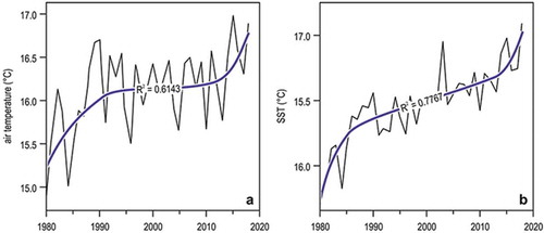
Figure 3. Surface isotherms of February in the Ligurian Sea. (a) Climatological means from the historical dataset 1906–1985. (b) Means for 1985–2006. Redrawn and modified from Bianchi et al. (Citation2012).
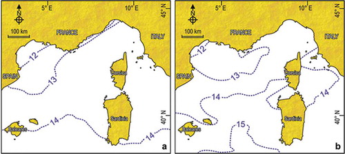
Figure 4. Surface circulation in the Ligurian Sea. (a) Scheme of the main current systems, with the steady Ligurian Circuit (colder) and the inflowing Tyrrhenian Current (warmer). (b) Satellite infra-red thermal imagery (AVHRR NOAA 9): the whitest areas are the warmest.
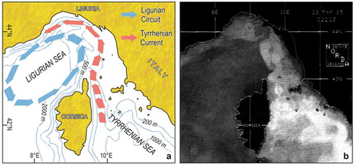
Figure 5. Trends in southern species occurrence in the Ligurian Sea. (a) Number of native or non-indigenous southern species recorded by diving in several localities of Liguria per 5-year period; the curves represent the second degree polynomial fits. (b) Yearly trends in the number of native or non-indigenous southern species in Genoa sites regularly monitored. The best fit is linear for native southerners and exponential for non-indigenous species. Redrawn and modified from Bianchi et al. (Citation2018a).
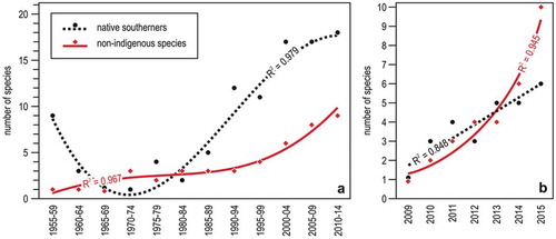
Figure 6. Examples of invertebrate mortality in the Ligurian Sea. (a) Necrosis in the sponge Spongia officinalis (Portofino, 5 m depth). (b) Partial mortality of the scleractinian coral Cladocora caespitosa (Portofino, 10 m depth). (c) Branch necrosis in the gorgonian Eunicella cavolini (Portofino, 30 m depth). (d) Empty shell, still in living position, of the bivalve Pinna nobilis killed by the pathogen Mycobacterium (Bergeggi, 15 m depth).
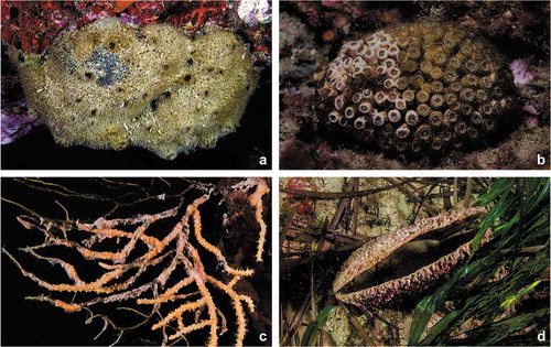
Figure 7. The heatwave of summer 1999 and gorgonian mortality in the Ligurian Sea. (a) Trend in sea water temperature at 0 m and 32 m depth, between August and October. Lines are weekly averages, bands the confidence limits (± 95%) obtained from the secular (1909–1987) trend calculated on Ligurian Sea records. (b) Percentage of partially (grey) and totally (black) dead colonies in three common gorgonian species. Redrawn and modified from Cerrano et al. (Citation2000).
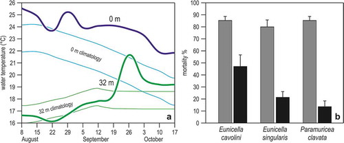
Figure 8. Phenology of the mucilage event of 2018 at Portofino. (a) Abundance of mucilage aggregated according to time and depth. Circles are roughly proportional to mucilage cover. Approximate positions of summer thermoclines are also indicated. (b) 100% cover of mucilage aggregates at about 20 m depth in July. (c) Mucilage filaments entangling the gorgonian Eunicella cavolini at about 30 m depth in August. (d) Mucilage filaments entangling the gorgonian Paramuricea clavata at about 40 m depth in September.
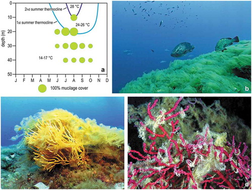
Figure 9. Two examples of fish species catched in the tuna trap (“tonnarella”) of Camogli. (a) The greater amberjack Seriola dumerili has been first recorded in the 1990s. (b) The bullet tuna Auxis rochei has halved in abundance with respect to the 1950s.
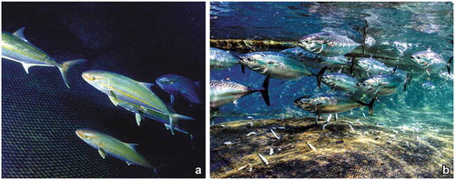
Figure 10. Changes in seagrass meadows of Liguria. (a) Time trend of Posidonia oceanica meadow extent since the mid of the XIX century, combining modelling, estimations, and quantitative cartographic measurements. The curve depicts the second degree polynomial fit of the data. (b) Time trend of the proportion of Cymodocea nodosa out of the total areal extent of seagrass meadows, and of the proportion of the linear extent of artificial structures on the coastline.
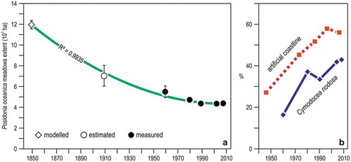
Figure 11. Trends in the Posidonia oceanica meadow at Monterosso. The curves depict the third degree polynomial fit of the data. (a) Yearly means (± se) of cover values, 1991–2006. (b) Discontinuous measures of mean shoot density (± se), 1991–2017. Data from Peirano et al. (Citation2011) and Regione Liguria (http://www.cartografiarl.regione.liguria.it/SiraQualMare/script/PubRetePuntoParam.asp?_ga=2.97453724.2042002155.1518772812-601063746.1517569932&fbclid=IwAR00qk1ShUaKXOxg0Hdi3lTtzAjMvUir-ryolOenpw9-v_yTP4wcI3wI2yk).
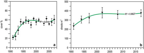
Figure 12. Changes in the Posidonia oceanica meadow of Bergeggi in 25 years. (a) Position of the meadow upper limit with respect to 1987. (b) Time trajectory of the meadow in the MDS ordination plane; pie diagrams illustrate the quantitative meadow composition. Redrawn and updated from Oprandi et al. (Citation2014a, Citation2014b).
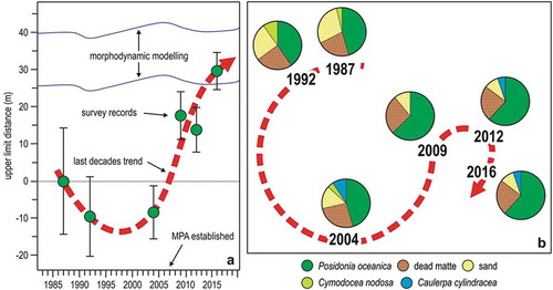
Figure 13. Change in the rocky reef communities of Portofino at about 10 m depth. (a) Sargassum vulgare and Dictyopteris polypodioides canopy in 1981. (b) Sarpa salpa grazing in a turf-dominated environment in 2009. Modified from Parravicini et al. (Citation2013).
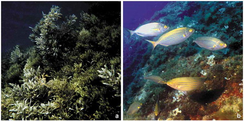
Figure 14. Change in the hydroid assemblage of Portofino reef. (a) Monthly variations in the total number of species in three years. (b) Corydendrium parasiticum, a species first recorded in 2018 in shallow waters (<5 m).
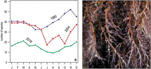
Figure 15. Compositional change in the rocky reef community of Mesco Shoal. Others include species whose cover has always been <5%.
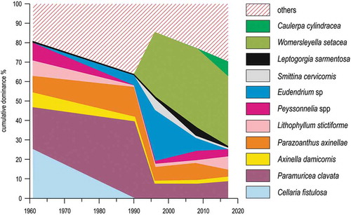
Figure 16. Ordination plot on the first two axes from Correspondence Analysis of epibenthic species cover data (82 species × 78 sampling quadrats) of Gallinara Island, in 1991, 2009, and 2016. Variance explained: 47.0%. All diagrams are in the same plane and have been split for ease of reading. Station-point centroids are identified by their depth (in meters). Lines illustrate the depth gradient.
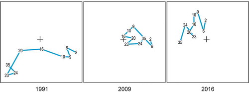
Figure 17. Selected examples of epibenthic species that changed their mean cover (± se) with time in Ligurian rocky reefs. Note logarithmic scale on y axis.
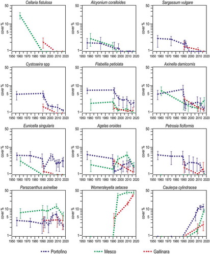
Figure 18. Selected examples of species that changed their depth range preference (mean ± se), going deeper with time, in Portofino rocky reefs.
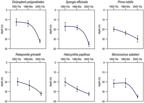
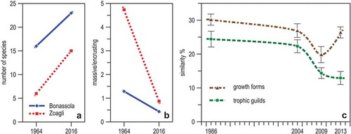
Figure 19. Change with time in the communities of Ligurian marine caves. (a) Number of sponge species in the two semi-submerged caves of Bonassola and Zoagli in 1964 and 2016. (b) Percent ratio of massive to encrusting sponge species in the same caves and in the same years. (c) Trends of average (± se) Bray-Curtis similarity among the sessile communities of the Bergeggi marine cave from 1986–2013, using morpho-functional descriptors. (a) and (b) from data in Costa et al. (Citation2018), (c) redrawn and modified from Montefalcone et al. (Citation2018).