Figures & data
Figure 1. Measurement of sponge body mechanical properties using the MTS Synergie 100 universal testing machine. (a) Montage of sponge in the tensile test. (b) Elongation-force curve: AB The rectilinear section of the curve; red point: maximum force value. (c) Montage of sponge in the 3-point bending test. (d) Force-deflection curve for five loading-unloading cycles, Q1 – energy dissipated within the first cycle; δ – deflection in the first cycle.
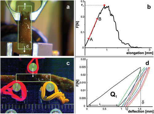
Figure 2. Image of Spongilla lacustris in its natural environment and reconstruction of a sponge base allowing it to be firmly attached to a substrate. (a) Image of sponge on the surface of concrete. (b) Projection of the 3D reconstruction of the sponge body; optical scan. (c) Developed surface of the sponge base adhering to the concrete surface.
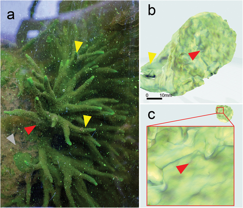
Figure 3. Reconstruction of Spongilla lacustris fragment based on the µCT images. (a) In situ image of the sponge colony and the fragment used for analysis (red frame). (b–e) Computer image reconstructions of the sponge skeleton based on the µCT (X radia Zeiss): (b) skeleton reconstruction in resolution 5.9834 µm/pixel; (c) skeleton reconstruction in resolution 2.508 µm/pixel; (d) skeleton reconstruction in resolution 0.95; (e) skeleton resolution 0.4424.
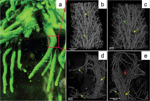
Figure 4. SEM EDS mapping of elements in megasclere and mesohyl of Spongilla lacustris body. (a) General view of the sponge body, topography, SE2 Everhart-Thornley detector, field of view 71 micrometers. (b–e) Corresponding chemical elements’ distribution 2D map of the analyzed object, energy-dispersive X-ray spectroscopy EDS: (b) carbon; (c) oxygen; (d) silicon; (e) sulfur.
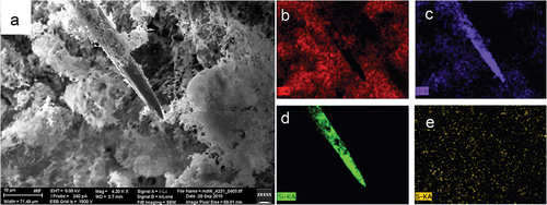
Figure 5. Image of Spongilla lacustris megascleres with a visible channel in the centrum in different imaging techniques. (a) SEM image, view of the sponge spicules, topography, SE2 Everhart-Thornley detector, field of view 112 micrometers, low-voltage imaging mode. (b) X-ray microscopy (c) CLSM confocal microscopy. (d) Light microscopy and histochemical methods (methylene blue staining).
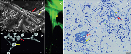
Figure 6. Reconstruction the spicule bundle of Spongilla lacustris skeleton with marked directions of individual megasclere based on µCT. (a) Branch with branchings. (b) Branch with color-marked angles of the megascleres according to the color scale (angle determined in relation to horizontal line). (c) Distribution of the angles between spicules.
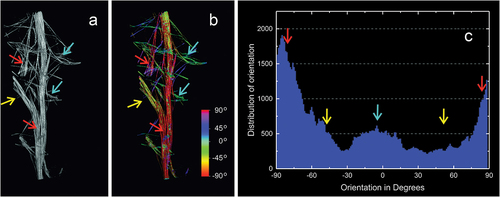
Figure 7. Reconstruction of individual beam and its branches based on µCT (X radia Zeiss) and places where megascleres emerge from the pinacoderm of Spongilla lacustris. (a) Visualization using Neurite Tracer and OrientationJ at various angles, red arrow – one of the central branches selected for analysis, green arrow – transverse crossbars beams. (b) Projection on the ground plane (red arrow – central beam; green arrows – transverse crossbars beams). (c–e) Places where megascleres emerge from the pinacoderm (blue triangles) and the location of the sponge skeleton branch (yellow circles).
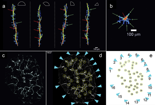
Table I. Measurement values of Spongilla lacustris skeletal elements obtained by analyzing images from X ray μCT.
Figure 8. Image of the intersection of spicule bundles in the siliceous-organic skeleton of Spongilla lacustris. (a) Methylene blue stained cross-section. (b) Reconstruction of the µCT image (0.95 µm) of beams and crossbars junction. (c) Image of the two beams and crossbars in confocal microscopy image. (d) SEM image.
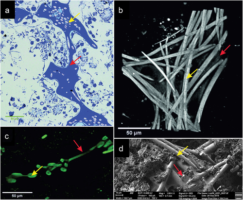
Figure 9. Cross-sections of the sponge and surface of Spongilla lacustris. (a–h) Cross-sections of the sponge 50 stack thick (~250 µm) with centrally arranged bundles of the main branch (dark nodes) and lateral branches, and spikes extending above the surface of the sponge. (i) Surface of sponge body with spikes constituting the ends of the side arms of the skeleton (SEM). (j) Surface of sponge body (in situ photography).
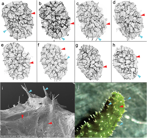
Figure 10. Imaging of the sponge Spongilla lacustris skeleton, based on SEM (Hitachi Uhr FE-SEM Su 8010); optical microscopy with methylene blue dying; µCT computed Tomography (X radia Zeiss) and CLSM technic. (a) The megascleres with the multilayer membrane on the surface. (b) Cross-sections of sponge body with megascleres and multilayer coating. (c) Reconstruction of sponge skeleton’s branch and lateral branching with marked enclosed layer. (d) Megascleres and autofluorescent layer. Megascleres central beam with marked beam forks and multilayer membrane.
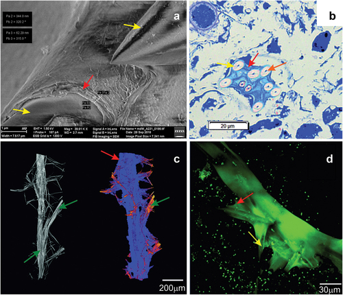
Figure 11. SEM image of protocolagen fiber in pinacoderm of the sponge Spongilla lacustris. (a) Pinacoderm surface with pores (red box indicates analyzed surface, SEM image by Jagna Karcz). (b) Fragment of pinacoderm utilized to analysis. (c) Analysis of fiber direction in the pinacoderm (calculated angles visualized according to color scale). (d) Distribution of fiber orientation in the pinacoderm.
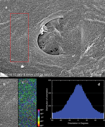
Figure 12. Diagram of the Spongilla lacustris structure. (a) Surface of the sponge’s base adhering to the concrete substratum. (b) Reconstruction of sponge spicular skeleton’s bundle and branch with marked layer. (c, d) Places where megascleres emerge from the pinacoderm. (e) Surface of the pinacoderm (body surface). (f) One of the central branches selected for analysis, projected onto the ground plane. (g, h) Main branch with the branching region.
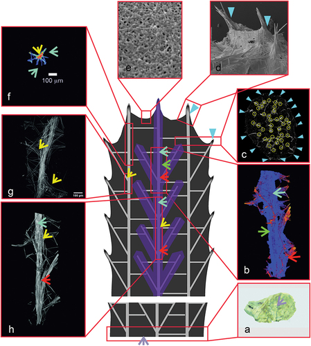
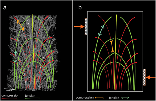
Figure 13. Graphical representation of the effect of drag force on a sponge skeleton. (a) Force diagram with the image of sponge skeleton reconstructed using µCT image. (b) Interactions occurring in the sponge skeleton as a result of drag force.