Future effects of small hive beetle, Aethina tumida, on honey bee colony in Turkey based on temperature factor using a mathematical model

Figures & data

Figure 1. Bifurcation diagram of the coexistence state for different system parameters. The black line indicates the sign change of the eigenvalues.

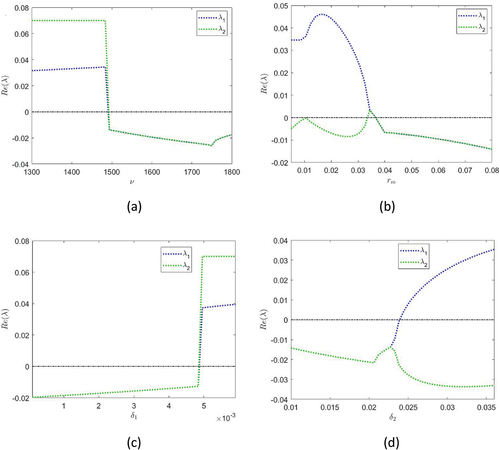
Figure 2. NOAA Climate.gov graph of annual surface temperature from 1880 to 2020, based on National Centers for Environmental Information (NCEI) data (NOAA National Centers for Environmental information 2022). Using the Matlab curve fitting toolbox’s linear approximation, the thick red line indicates a linear approximation to field data determined between the relevant years.

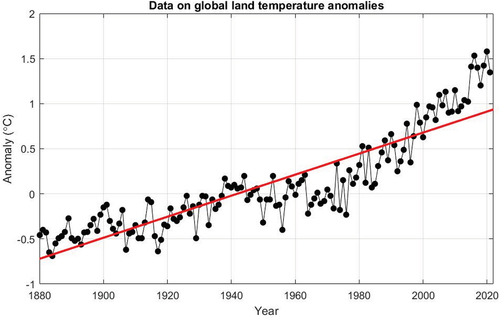
Figure 3. (a) Sketch of brood temperature versus time (red), where the lower and upper temperature are assumed to be 32 and 36°C, respectively; (b) sketch of SHB growth (green) over time.

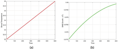
Figure 4. Honey bee population (blue) and SHB population (black) against time obtained for given temperature function as in Figure 2(a). The rest of the parameters are the same as in the text. The figure shows the effect of the maximum developmental rate of SHB on the system dynamics for (a) $r_m=0.01$, (b) $r_m=0.02$, (c) $r_m=0.03$ and (d) $r_m=\mathrm{0.08.}$.

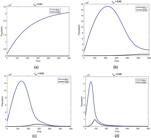
Figure 5. Honey bee population (blue) and SHB population (black) against time obtained for a given temperature function, as in Figure 3(a). The rest of the parameters are the same as in the text. The effect of the maximum developmental rate of SHB on the system dynamics is fixed and the different SHB invasion rates γ are compared as (a) $\gamma ={10}^{-8}$ (b) $\gamma ={10}^{-7},$ (c) $\gamma ={10}^{-6}$ and (d) $\gamma ={10}^{-5}.$

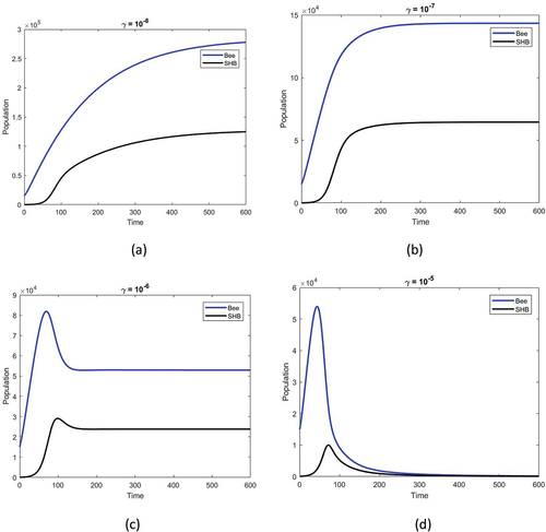
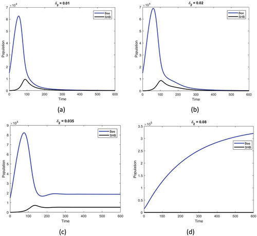
Figure 6. Honey bee population (blue) and SHB population (black) against time obtained for a given temperature function, as in Figure 2(a). The rest of the parameters are the same as in the text. The effect of the SHB death rate increases with an increase in temperature as (a) ${\delta }_2=0.01,$ (b) ${\delta }_2=0.02,$ (c) ${\delta }_2=0.035\hspace{0.17em}$ and (d) ${\delta }_2=0.08.$

NOAA National Centers for Environmental information. 2022. Climate at a glance: Global time series. Available: https://www.ncdc.noaa.gov/cag/. Accessed Feb 2022 10.

 Google Scholar

Data availability statement

The data that support the findings reported in this study are available from the corresponding author upon reasonable request.