
Figures & data
Figure 1. Location and genetic makeup of 33 wild sampling sites in the northern Apennines (Italy) and four hatcheries (indicated in the bottom-right map). Pie charts, proportional to sample size, indicate the frequency and the geographic distribution of three genetic classes defined by combining information from the LDH-C1 genotype and the D-loop haplogroup: “native” = LDH-C1*100/*100 and an AD, ME or MA haplotype; “exotic” = LDH-C1*90/*90 and an AT haplotype; “hybrid/introgressed” = mixed genetic profiles. Site abbreviations are defined in ; the FCNP area is shown in pale green; dotted lines mark boundaries of major drainage basins; the purple rectangle indicates the study area in the bottom-right map.
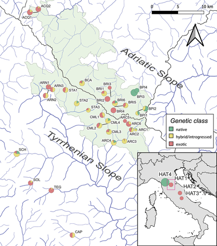
Table I. Detailed information on 33 sampling sites and 4 hatcheries of (Mediterranean) brown trout in northern Italy: river catchment and sampling locality; administrative region and protected area (FCNP = Foreste Casentinesi National Park); Apennine slope (Slope); elevation above the sea level (Elev); approximated geographic coordinates (datum = WGS84); sample size (N); sample size for STR-based analyses.
Table II. Genetic information obtained for 699 brown trout from the monitored 33 sampling sites and 4 hatchery stocks: LDH-C1 nuclear gene genotypes; LDH-C1-based introgression rate (i.e., frequency of the exotic Atlantic LDH-C1*90 allele); mitochondrial D-loop haplotypes; D-loop-based introgression (i.e., frequency of the exotic AT haplogroup); genetic classes obtained combining the individual LDH-C1 genotype and the D-loop haplotype (“native” = LDH-C1*100/*100 and native haplotype; “exotic” = LDH-C1*90/*90 and AT haplotype; “hybrid/introgressed” = mixed genotypes). The Apennine slope and the sample size (N) are also shown.
Table III. Genetic diversity indices and results of demographic analyses for 12 brown trout sampling sites and 4 hatcheries (Site): observed (Ho) and expected (He) heterozygosity; the average number of alleles (An) and private alleles (Pa); allelic richness (Ar); probability (p) of a severe recent bottleneck as inferred by BOTTLENECK analysis according to IAM e TPM models. Standard errors (SE) are shown in parentheses when appropriate. The number of analyzed individuals at STR loci (NSTR) and the Apennine slope is also indicated for wild sites and the hatchery of Mediterranean trout.
Figure 2. Relationship (quadratic regression) between the frequency of the domestic-Atlantic LDH-C1*90 allele and measures of genetic diversity – allele richness (a), observed heterozygosity (b), based on 15 STR loc. For each model, R-squared, statistics, p-value, and 95% confidence intervals (in grey) are shown. Site abbreviations refer to ; colours distinguish between Adriatic FCNP sites (pale green), Tyrrhenian FCNP sites (aquamarine), Atlantic hatcheries (pale red) and the Mediterranean hatchery (violet).
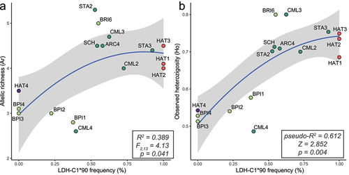
Figure 3. Non-metric multidimensional scaling (NMDS) of the population-pairwise genetic distance (Fst) matrix based on 15 STR loci. Wild sites/hatcheries, which abbreviations refer to , are grouped according to their geographic area of origin and coloured accordingly: Tyrrhenian Apennine slope; Adriatic Apennine slope; Atlantic (hatchery strains); Magra-Vara drainage basin (Mediterranean hatchery).
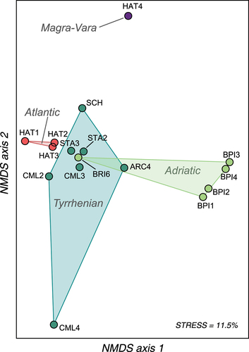
Figure 4. Results of the Bayesian clustering inference (independent allele frequencies) based on 15-STR genotypes of 272 brown trout from 12 wild sampling sites and four hatcheries in central-northern Apennines (Italy): the distribution of Evanno’s ∆K (a) and the log-likelihood probability (b) for increasing K values; barplots of individual assignment values according to the optimal clustering – K = 3 (c), K = 4 (d) and K = 5 (e). Site/hatchery abbreviations refer to .
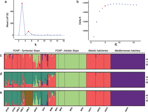
Figure 5. The distance tree generated by STRUCTURE and depicting genealogies among the 5 inferred genetic clusters (K = 5). Cluster colors refer to . Sites clearly assigned to a cluster (< 30% admixture) are indicated in parentheses – (*) note that “Tyrrhenian” refers to the geographic location of sites, rather than their genetic makeup (see text for details).
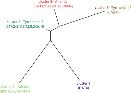
Table IV. Results from AMOVA hierarchical analyses examining the partitioning of genetic (15 STR loci) variance according to different hypothesized structures: (1) no structuring with one panmictic population (no groups); (2) geographic differentiation with four groups defined according to major geographic areas of origin; (3) optimal genetic clustering (3 and 5 groups, after removing substantially admixed sites that cannot be clearly assigned to a cluster) as revealed by STRUCTURE analyses. The amount of variation (%) explained by differences among groups, among populations within groups, and within populations, along with the statistical significance of p-values (*** = p < 0.001; ** = p < 0.01; * = p < 0.05; ns = p ≥ 0.05) are given.