
Figures & data
Figure 1. The basic architecture of a classic WiFi indoor fingerprinting system with machine learning as its positioning algorithm. This system has two phases: the off-line phase and the on-line phase. In the off-line phase, the WiFi fingerprinting signals, which are WiFi RSS data here, are collected, preprocessed, labelled and stored in the database. In the on-line phase, the RSS signals received by the user are compared with the signals in the database by the machine learning positioning algorithm to get the final location estimation. The basic architecture of deep learning based WiFi indoor fingerprinting system will be explained in and .
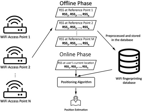
Table 1. An example fraction of the WiFi RSS data.
Figure 2. The structure of a deep neural network based on WiFi RSS for predicting the building where the user is in. In this structure, the input layer contains the original input. Layer 1 to layer 3 are the hidden layers. Layer 4, between hidden layers and the final output, is the output layer.
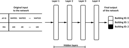
Figure 3. The basic architecture of ANN and its neuron.
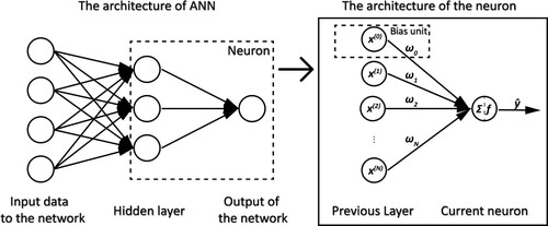
Figure 4. The structure of an AE network where the encoder part compresses the input data, while the compressed data is decoded by the decoder part.
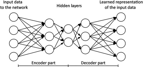
Figure 5. A real example of CNN architecture introduced in Sinha and Hwang (Citation2019).

Figure 6. The basic structure of RNN. The recurrent layer utilizes the current input element input t, and the state from the last layer state t, and then it generates a temporary output output t and a new state, state t+1, which represents the information of what it has seen so far. Through the recurrent layers, RNN is able to extract features from time-series data or sequence data.
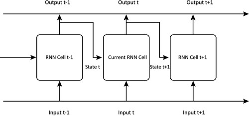
Figure 7. The basic structure of GAN. The generator and the discriminator are trained at the same time. The generator network generates data as similar to the real data as possible and the discriminator network outputs the similarity between the real data and the generated data.
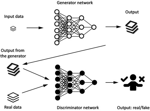
Table 2. Comparison of the covered WiFi-based indoor positioning systems using Deep Learning as a feature extraction method.
Table 3. The RSS-based systems that achieve sub-metre level MDE.
Table 4. Comparison of the covered WiFi-based indoor positioning systems using Deep Learning as a prediction method.
Figure 8. Hidden layers are the layers between input layer and output layer. The number of hidden layers could vary from only one to hundreds.
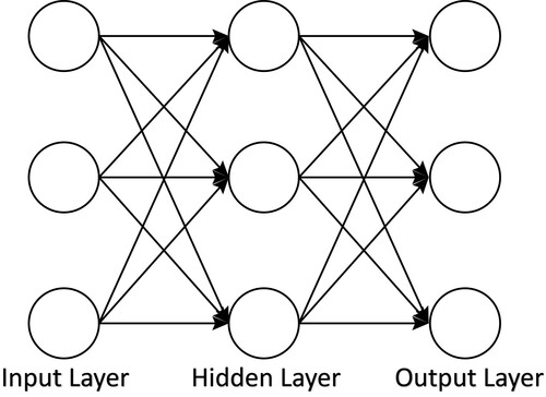
Figure 9. The general process of WiFi-based indoor positioning systems employing deep learning as a feature extraction method. Please note that the difference between deep learning and neural networks is identified in this figure. While in the comparisons, all the different neural networks adopted by covered systems will still be compared whether they are deep neural networks or simple neural networks.
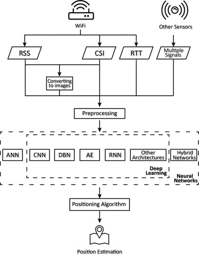
Figure 10. The structure of the system proposed by Qi et al. (Citation2018). The RSS data are preprocessed by PCA and then fed into multiple ELM classifiers. The results from these classifiers are used to predict the location of the user.
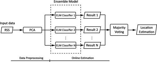
Figure 11. The structure of the system proposed by Belmonte-Hernández et al. (Citation2019). The input data of the system are the RSS signals of XBee, Bluetooth and WiFi. The system also adopts information from Step and Velocity Estimator and Yaw estimation in the feature vectors. The ANN is then used to perform fingerprinting estimation and generate the probabilities of the user's being at a specific location. The Gaussian filter detects the outliers from the ANN's output and then passes the processed data to the particle filter. The particle filter estimates the user's final location based on the realistic movement model.
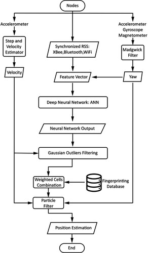
Figure 12. The architecture of the deep learning network in StoryTeller.
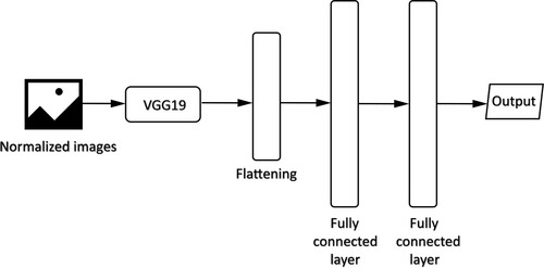
Figure 13. The DeepFi system. The normalized CSI data are separated according to their location. The deep learning method uses the CSI information to reconstruct the WiFi fingerprints with the weights of all the locations. Probabilistic methods are then used to estimate the user's location given a test CSI.
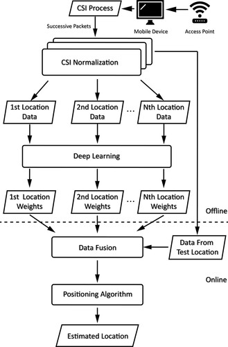
Figure 14. The neural network structure in DeepFi. The encoder part of the neural network labelled as ‘Pre-training’ in the figure is used to perform noise reduction and dimension reduction of the input data. K1, K2, K3 and K4 denote the number of neurons in the first, second, third, and fourth hidden layer, respectively.
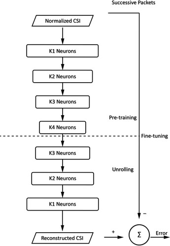
Figure 15. The boxplot shows RMSE results of the systems that use deep learning as feature extraction methods. It can be seen from the figure that utilizing more than one neural network could improve the RMSE results for a WiFi indoor positioning system. For instance, the best RMSE of 0.339 m is given by W. Zhang et al. (Citation2016) which uses the combination of DNN and SDAE to extract features from the input data.
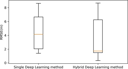
Figure 16. Comparison of the indoor positioning systems based on different WiFi signals. CSI-based systems could perform better, more stable and more accurate positioning estimation than RSS-based ones.
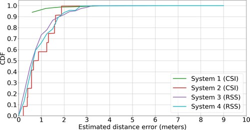
Figure 17. The boxplot of the MDE results for covered systems based on different inputs. Though WiFi RSS-based systems using deep learning as feature extraction methods could achieve generally better results than those based on CSI, the variation of their MDEs is larger. It is worth noticing that the best three RSS-based systems all utilize signals from other sensors (e.g. Inertial Measurement Unit (IMU)) to improve their positioning stability.
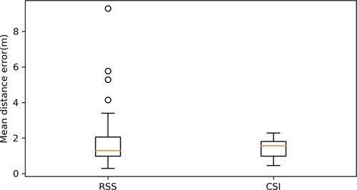
Figure 18. The MDE boxplot shows the effect of using different neural networks to extract features. Both ANN and CNN perform generally better than other neural networks. The mean MDE of indoor positioning systems using ANN is 1.607 m while that of CNN is 1.343 m. It is demonstrated in the boxplot that ANN, as a feature extraction method with less computational cost compared to CNN, is able to effectively generate meaningful information from the input data.
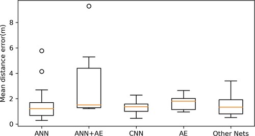
Figure 19. The general process of WiFi indoor positioning systems employing deep learning as prediction methods. Please note that the difference between deep learning and neural networks is identified in this figure. While in the comparisons, all the different neural networks adopted by covered systems will still be compared whether they are deep neural networks or simple neural networks.
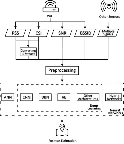
Figure 20. The architecture of the neural network proposed by Koike-Akino et al. (Citation2020). ‘BN’ represents batch normalization which is a deep learning approach to normalize the data. This network utilizes the residual blocks to maintain the residual gradient from the input data and perform location-only classification, simultaneous location-and-orientation classification and direct coordinates estimation based on different output layers.
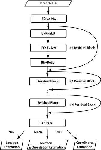
Figure 21. The transformation from the RSS signals to a 2D-image data. Each greyscale image is converted from 256 RSS signals. The brightness of the pixel in the image represents how strong the corresponding RSS is. The black dots in the image indicate that RSS from the corresponding APs can not be received.
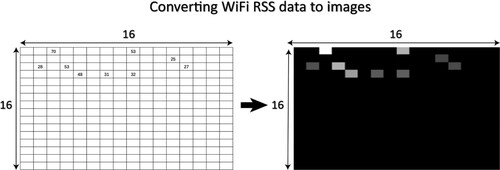
Figure 22. The architecture of the CNN in Sinha and Hwang (Citation2019). This neural network contains 4 convolutional layers and fully connected layers to perform classification.
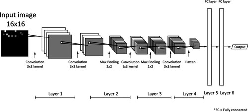
Figure 23. The architecture of the 1D-CNN in C. H. Hsieh et al. (Citation2019).
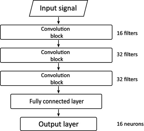
Figure 24. The structure of the DNN proposed by Kim, Wang, et al. (Citation2018). The system treats the multi-label classification questions as multi-class classification ones. Since it predicts the building, floor and location via different output layers, the system becomes scalable and flexible and could be implemented easily in different indoor positioning scenarios.
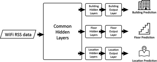
Figure 25. The boxplot shows the floor hitting rate results for systems using deep learning as a prediction method. The papers are grouped according to the main types of neural networks they use. It is illustrated in the boxplot that ANN and DBN are better in floor-level prediction while the variances in both groups are comparatively higher. Among the top 5 floor prediction systems with floor hitting rate above 98, 3 of them apply ANN.
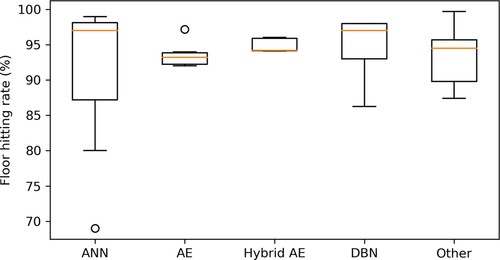
Figure 26. The boxplot shows the zone hitting rate results for systems using deep learning as prediction method. This boxplot mainly compares the effect of using different WiFi signals as the input. CSI is more stable than RSS signals or even hybrid RSS input signals. The hybrid RSS input signals mean a combination of RSS and signals from other sensors (e.g. magnetometre, accelerometre, and Bluetooth).
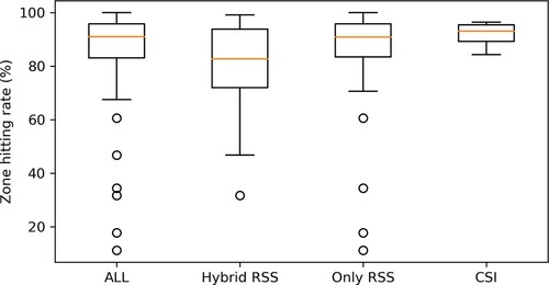
Figure 27. The boxplot shows the zone hitting rate results for systems using deep learning as a prediction method. This boxplot mainly compares the effect of using different neural networks. Though some systems based on ANN could achieve the best result in the comparison, the variance of all ANN systems is astonishingly large which represents the instability of ANN systems. It could be deduced by the boxplot that CNN is generally better in zone predicting.
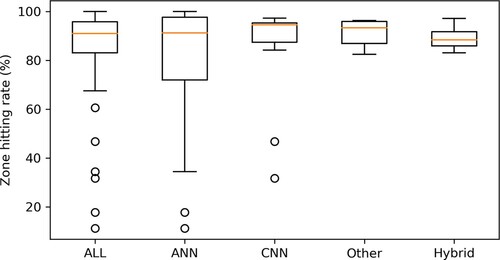
Table 5. The top 3 zone predicting systems that utilize deep learning as prediction solution.
Figure 28. The boxplot of MDE results from systems using deep learning as the prediction method. This boxplot aims to compare the effect of using different WiFi signals as the input to the positioning system. CSI could provide more accurate and stable results about the user's location, while hybrid RSS signals could largely improve the RSS-based positioning accuracy.
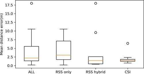
Figure 29. The effect of using CSI amplitude or CSI phase as the input to the neural network. Either for the general performance or the variance in the results, CSI amplitude is a better choice for indoor positioning systems to get more accurate position estimation.
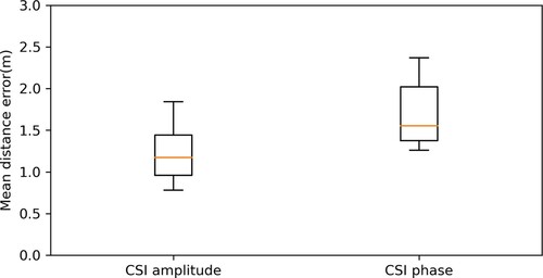
Figure 30. The boxplot compares the MDE from systems using different neural networks. Due to the comparatively good performance and relatively higher number of systems using CNN, it could be derived from the figure that CNN is the best neural network to perform coordinates prediction.
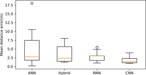
Table 6. All systems reach the sub-metre level MDE while utilizing deep learning as prediction method.