Texture recognition under scale and illumination variations

Figures & data

Figure 1. Unilateral contextual neighbourhood $I_r$ of sixth-order used for CAR model. X marks the current pixel, the bullets are pixels in the neighbourhood, the arrow shows movement direction, and the grey area indicates acceptable neighbourhood pixels.

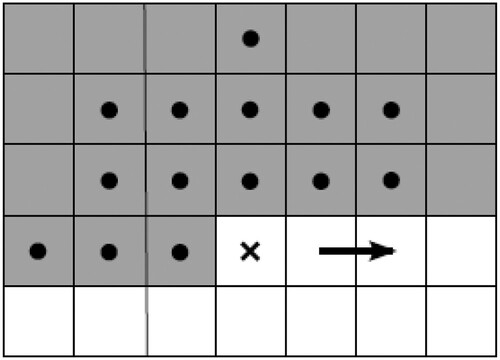
Figure 2. The texture analysis algorithm flowchart uses 2D random field models; the K-L transformation step is optional.

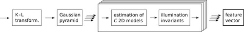
Table 1. The sizes of feature vectors of compared textural features.

Colour histogram	384	LBP${}_{16,2}^u$, gray	243
Gabor, gray	48	LBP${}_{16,2}^u$, colour	729
Gabor, colour	144	LBP${}_{8,1+8,3}$, gray	512
Opponent Gabor	252	LBP${}_{8,1+8,3}$, colour	1536
2D CAR-KL	1515	2D CAR-KL (K = 4)	1212
2D CAR	1515

Figure 5. The appearance of patterns from the UEA database with varying scales, from the left, the scale factor is 50%, 60%, 75%, 90%, and 100%.

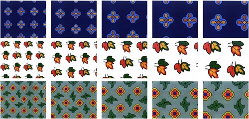
Figure 11. The appearance of two veneers from the Wood UTIA BTF database in varying scales, from the left, the scale factor is 50%, 60%, 75%, 90%, and 100%.

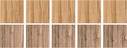
Figure 3. Examples of patterns included the UEA database.

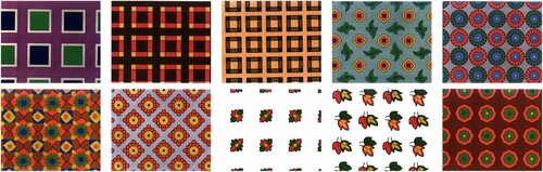
Figure 4. The appearance of patterns from the UEA database with varying illumination spectra (3 columns on the left) and additional acquisition devices (2 columns from the right).

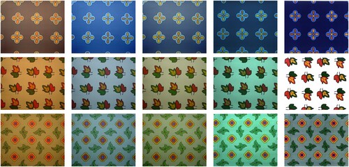
Table 2. Classification accuracy [%] averaged over all scales and illumination conditions on the UEA dataset.

No. of training samples	1	3	6
Colour histogram	15.3	23.2	32.6
Gabor, gray	29.6	44.5	53.2
Gabor, colour	33.9	46.2	59.7
Opponent Gabor	44.0	61.0	70.1
LBP${}_{16,2}^u$, gray	18.4	35.0	45.8
LBP${}_{16,2}^u$, colour	17.7	31.2	41.2
LBP${}_{8,1+8,3}$, gray	13.9	28.8	38.2
LBP${}_{8,1+8,3}$, colour	14.1	28.2	38.1
2D CAR-KL (K = 4)	43.1	58.2	67.0
2D CAR-KL	48.4	62.8	70.2
2D CAR	52.1	66.2	73.0

Note: Columns display results for the increasing number of training samples per class.

Figure 6. The illustration of the classification accuracy [%] progresses with decreasing scale differences among training and test sets (UEA dataset). On the left, for one training sample, and on the right, for six training samples per class.

Figure 7. The classification accuracy [%] for all combinations of scales among training and test sets on the UEA dataset, one training sample per class was used.

Figure 8. Classification accuracy [%] on the UEA dataset with one training sample, on the left for the training sample with the scale factor of 1 and on the right with the scale factor of 0.5.

Figure 9. Examples of wood veneers included the Wood UTIA BTF database.

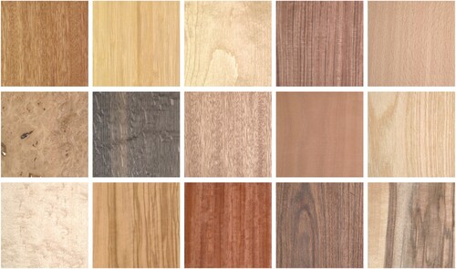
Figure 10. The illustration of the appearance of four veneers from the Wood UTIA BTF database in varying illumination directions. The left column is illuminated from the surface normal, and the direction of illumination tilt increases to the right: 0, 30, 60, 60, and 75 degrees, illumination azimuth is 0, 90, 180, 252, and 345 degrees, respectively.

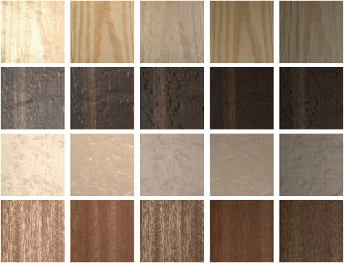
Table 3. Classification accuracy [%] averaged over all scales and illumination angles on the Wood UTIA BTF dataset.

No. of training samples	1	3	6
Colour histogram	10.6	19.7	28.6
Gabor, gray	11.9	20.2	25.1
Gabor, colour	18.0	28.6	36.8
Opponent Gabor	24.0	36.4	44.3
LBP${}_{16,2}^u$, gray	7.2	11.0	13.3
LBP${}_{16,2}^u$, colour	10.9	16.0	19.6
LBP${}_{8,1+8,3}$, gray	10.8	15.8	19.3
LBP${}_{8,1+8,3}$, colour	13.3	21.0	25.6
2D CAR-KL (K = 4)	39.9	55.7	64.3
2D CAR-KL	45.4	61.4	69.4
2D CAR	32.8	47.1	55.7

Note: Columns display results for the increasing number of training samples per class.

Figure 12. Classification accuracy [%] progresses with decreasing scale differences among training and test sets (Wood UTIA BTF). On the left, for one training sample, and on the right, for six training samples per class.

Figure 13. The classification accuracy [%] for all combinations of scales among training and test sets on the Wood UTIA BTF dataset, one training sample per class was used.

Figure 14. Classification accuracy [%] on the Wood UTIA BTF dataset with one training sample, on the left for the training sample with the scale factor of 1 and on the right with scale factor of 0.5.

Table 4. Classification accuracy [%] is shown for different illumination tilts (declination angle from the surface normal) without any scale variation (Wood UTIA BTF).

Illumination tilt [deg]	30	60	75	avg.
Colour histogram	5.6	1.7	1.5	3.0
Gabor, gray	26.9	10.3	5.5	14.2
Gabor, colour	30.2	13.4	5.4	16.3
Opponent Gabor	50.1	26.1	14.9	30.8
LBP${}_{16,2}^u$, gray	46.8	16.3	9.2	24.1
LBP${}_{16,2}^u$, colour	52.7	20.0	12.9	28.5
LBP${}_{8,1+8,3}$, gray	55.4	22.1	12.1	29.9
LBP${}_{8,1+8,3}$, colour	55.8	25.2	13.6	31.5
2D CAR-KL (K = 4)	76.4	54.6	32.4	54.5
2D CAR-KL	83.3	62.9	42.1	62.8
2D CAR	74.7	49.7	25.8	50.1

Note: The training sample is illuminated from the surface normal direction.