An extended sparse max-linear moving model with application to high-frequency financial data

Figures & data

Figure 1. Left side: Signature pattern of MM(1) process with . It is shown in Zhang and Smith (2010) that signature patterns will occur infinitely many times in a moving maxima processes. Right side: The loading constant α is replaced with a uniform random variable on the interval [0, 1] to remove the signature pattern.

Figure 2. Simulation of models (4(4) ) (left) and (5(5) ) (right) with size = 1000, (C, ψ, β, τ) = (0.001, 2, 1.5, −0.5) and α = (0.5, 0.3, 0.2). The horizontal lines are the 90th percentiles.

Figure 3. Simulation of model (4(4) ) with size = 1000, (β, τ) = (1.5, −0.5) and α = (0.5, 0.3, 0.2). Left side: First 50 realisations, t = 1 : 50. Right side: 901st to 950th realisations, t = 901: 950.

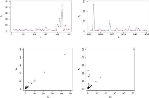
Figure 4. Simulation of models (4(4) ) (left) and (5(5) ) (right) with size = 1000, (C, ψ, β, τ) = (0.001, 2, 0.7, 0.5) and α = (0.5, 0.3, 0.2). The horizontal lines are the 90th percentiles.

Figure 5. Simulation of model (4(4) ) with size = 1000, (β, τ) = (0.7, 0.5) and α = (0.5, 0.3, 0.2). Left side: First 50 realisations, t = 1 : 50. Right side: 901st to 950th realisations, t = 901: 950. (Y₃₀, Y₉₀₄, Y₉₁₈, Y₉₄₃) = (110.2, 36749.2, 4545.1, 320.9) are out of the y-axis limits.

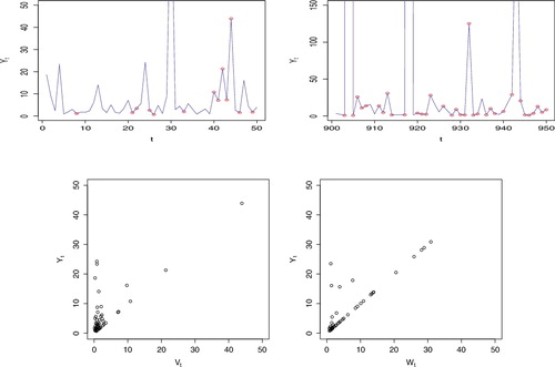
Figure 6. Simulation Result 2.1: Graph of MCMC results for all parameters of model (5(5) ), showing time plot, estimated posterior distribution and autocorrelation.

Table 1. Results of estimation for simulation example of model (5(5) ).

θ	True	Mean	Std. Dev.	θ0.5	[θ0.025, θ0.975]	Acc. Rate
C	0.001	0.00102	3.6e-05	0.00102	[0.00095, 0.00109]	0.3972
ψ	2.0	2.0289	0.0576	2.0245	[1.9285, 2.1555]	0.3984
β	1.5	1.4900	0.2067	1.4745	[1.1178, 1.9363]	0.3747
τ	−0.5	−0.6314	0.1570	−0.6188	[−0.9873, −0.3626]	0.3719
α1	0.5	0.5043	0.0660	0.5012	[0.3764, 0.6377]	0.2664
α2	0.3	0.3125	0.0619	0.3138	[0.1927, 0.4298]	0.2664
α3	0.2	0.1831	0.0581	0.1850	[0.0654, 0.2967]	0.2664

Table 2. Results of convergence test for simulation example of model (5(5) ).

θ	C	ψ	β	τ	α1	α2	α3
	1.00067	1.00036	1.00067	1.00052	1.00006	1.00002	1.00005

Table 3. Results of sensitivity analysis for simulation example of model (5(5) ).

		Mean		Median
θ	True	Logarithmic	Uniform	Logarithmic	Uniform
C	0.0010	0.00102	0.00102	0.00102	0.00102
ψ	2.0	2.0289	2.0286	2.0245	2.0232
β	1.5	1.4900	1.5158	1.4745	1.5133
τ	−0.5	−0.6314	−0.6516	−0.6188	−0.6357
α1	0.5	0.5043	0.5035	0.5012	0.5021
α2	0.3	0.3125	0.3133	0.3138	0.3139
α3	0.2	0.1831	0.1830	0.1850	0.1812

Table 4. Results of estimation for 500 simulation examples, using median values of the parameters from each simualtion. [Int. C.P. means Interval Coverage Probability.]

θ	True	Mean	Std. Dev.	[θ0.025, θ0.975]	95% Int. C.P.
C	0.0010	0.00102	4.4e-05	[0.00093, 0.00111]	0.964
ψ	2.0	2.0618	0.0759	[1.9393, 2.2316]	0.950
β	1.5	1.5263	0.2931	[1.0163, 2.1141]	0.939
τ	−0.5	−0.6450	0.1833	[−1.0707, −0.3086]	0.979
α1	0.5	0.5025	0.0615	[0.3833, 0.6262]	0.975
α2	0.3	0.2947	0.0533	[0.1910, 0.3947]	0.981
α3	0.2	0.2026	0.0555	[0.0959, 0.3159]	0.960

Table 5. Results of estimation for simulation example of model (5(5) ).

θ	True	Mean	Std. Dev.	θ0.5	[θ0.025, θ0.975]	Acc. Rate
C	0.0012	0.00122	5.9e-05	0.00123	[0.00107, 0.00131]	0.3761
ψ	1.5	1.6163	0.1951	1.6444	[1.1851, 1.9419]	0.4148
β	0.7	0.6766	0.1214	0.6436	[0.5261, 1.0192]	0.3748
τ	0.5	0.4647	0.0519	0.4591	[0.3757, 0.5740]	0.3635
α1	1/3	0.1851	0.1285	0.1623	[0.0092, 0.4852]	0.4685
α2	1/3	0.3921	0.1712	0.3910	[0.0710, 0.7359]	0.4685
α3	1/3	0.4226	0.1725	0.4202	[0.0786, 0.7686]	0.4685

Figure 7. Intra-daily maxima of the US Dollars vs. Japanese Yen 3-minute negative log-returns. The horizontal line is the 90th percentile.

Figure 8. Real data analysis of USD vs JPY: Graph of MCMC results for transformation parameters of model (5(5) ), showing time plot, estimated posterior distribution and autocorrelation.

Figure 9. Real data analysis of USD vs JPY: Graph of MCMC results for alpha parameters of model (5(5) ), showing time plot, estimated posterior distribution and autocorrelation.

Figure 10. Quantile-quantile plots using estimated mean values on left and median values on right.

Table 6. Results of estimation for real data example of intra-daily maxima of 3-minute negative log-returns of USD vs. JPY.

θ	Mean	Std. Dev.	θ0.5	[θ0.025, θ0.975]	Acc. Rate
C	8.84e-04	2.78e-05	8.84e-04	[8.31e0-4, 9.39e0-4]	0.3959
ψ	2.0448	0.0641	2.0406	[1.9264, 2.1825]	0.3926
β	1.3605	0.1507	1.3534	[1.0768, 1.6860]	0.3595
τ	−0.7200	0.1625	−0.7062	[−1.0650, −0.4444]	0.3805
α1	0.2989	0.1048	0.2973	[0.0938, 0.5059]	0.2533
α2	0.1822	0.0966	0.1778	[0.0180, 0.3861]	0.2533
α3	0.1115	0.0775	0.0996	[0.0052, 0.2938]	0.2533
α4	0.1323	0.0851	0.1200	[0.0077, 0.3267]	0.2533
α5	0.0959	0.0710	0.0818	[0.0039, 0.2623]	0.2533
α6	0.1789	0.0975	0.1732	[0.0138, 0.3879]	0.2533

Figure A1. Simulation result: Graph of MCMC results showing rapid fluctuation of parameters.

Figure A2. Simulation result: Graph of MCMC results showing scatter plot of parameters.

Figure A3. Unit Fréchet density (left) and Fréchet(β, 1, τ) density (right). Left: β = 1.5 and τ = −0.5. Right: β = 0.7 and τ = 0.5.

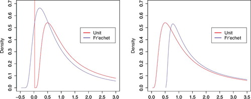
Figure A4. Simulation Result 2.2: Graph of MCMC results for all parameters of model (5(5) ), showing time plot, estimated posterior distribution and autocorrelation.

Zhang, Z., & Smith, R. L. (2010). On the estimation and application of max-stable processes. Journal of Statistical Planning and Inference, 140, 1135–1153.

 Web of Science ®Google Scholar