Semiparametric Bayesian analysis of high-dimensional censored outcome data

Figures & data

Figure 1. Estimated mean versus true mean of log-survival time for the n = 10, 000 individuals considered in the simulation study.

Figure 2. Posterior densities of σ (top) and τ (bottom) for the simulation study. The true parameter values are σ = 0.05 and τ = 0.4.

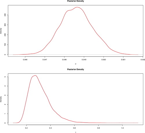
Table 1. Computational time comparison on simulated data.

Method	User time	System time	Elapsed time
Data quashing strategy applied	7654.6 sec	3 sec	7742.29 sec
No ata uashing trategy applied	22971.35 sec	92.08 sec	23206.64 sec

Figure 3. Posterior densities of the factor effect of black (top) and American Indian (bottom) races for SEER breast cancer New Mexico data.

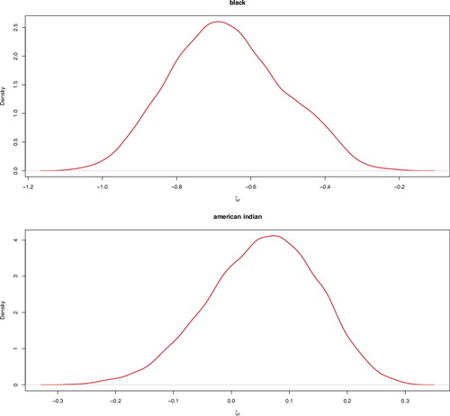
Table 2. 95% posterior credible intervals of selected parameters for the New Mexico breast cancer data.

		95% posterior credible interval
Parameter	Interpretation	Lower limit	Upper limit
β1	Patient age at diagnosis	−0.014	−0.009
β2	Calendar year of diagnosis	0.022	0.030
ζ2	Race : African American	−0.941	−0.364
ζ3	Race : Native American	−0.141	0.222
χ2	Tumor grade 2	−1.020	−0.820
χ3	Tumor grade 3	−1.869	−1.657
χ4	Tumor grade 4	−2.204	−1.751
χ3 − χ4	Difference between tumor grade 3 and 4	−0.047	0.433
K	Number of latent DP clusters	52	83
σ	AFT error s.d.	0.543	0.573
τ	DP base distribution s.d.	1.849	3.135
ση	CAR s.d.	0.225	0.509

Figure 4. Posterior densities of the factor effect of tumor grade 2 at diagnosis (top) and tumor 4 at diagnosis (bottom).

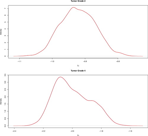
Figure 5. Estimates of the county-specific random effects for New Mexico. The labels are the county names.

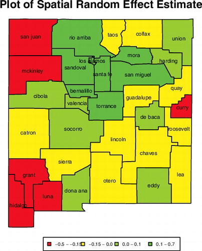
Figure 6. Standard errors of the county-specific random effects for New Mexico. The labels are the county names.

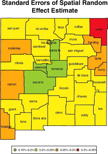
Figure 7. Posterior density of the individual-specific error distribution F defined in Equation (11(11) ). See the text for the interpretation of F. The narrow lines represent margins of 2 posterior standard deviations.

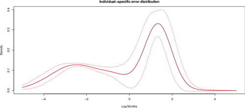
Table 3. Mixed effects cox regression for the New Mexico breast cancer data.

	95% posterior credible interval
Risk factor	Lower limit	Upper limit
Patient age at diagnosis	0.006482	0.011040
Calendar year of diagnosis	−0.038927	−0.031033
Race : African American	0.277142	0.730987
Race : Native American	−0.107270	0.267932
Tumor grade 2	0.725362	0.958409
Tumor grade 3	1.320884	1.549013
Tumor grade 4	1.125061	1.520721
Difference of Tumor grade 3 and 4	0.028292	0.195823