Shape-constrained semiparametric additive stochastic volatility models

Figures & data

Figure 1. Estimated autoregressive function f for the unleveraged SV models based on a single simulated dataset. The dashed line in each graph shows the true functional form of f and the solid lines represent the posterior average of f as well as the 95% credible bands. For the semiparametric models SC-SV and SP-SV, the 20-knot-interval version is presented.

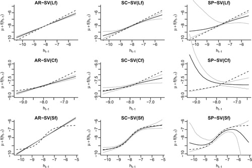
Table 1. For the three true unleveraged SV models (Lf , Cf and Sf ), a summary of the MSE and MAE of the log volatilities, $\{h_t{\}}_{t=1}^N$, obtained from fitting five different SV models. The averages and standard errors are multiplied by 100, and are based on 200 replicate series.

True Model		Fitted Models
		AR-SV	SC-SV(10)	SP-SV(10)	SC-SV(20)	SP-SV(20)
Lf
Average (s.e.)	MSE	36.3(0.2)	36.7(0.2)	40.2(0.4)	36.9(0.2)	43.2(0.6)
	MAE	47.9(0.1)	48.2(0.1)	50.4(0.3)	48.3(0.1)	52.2(0.3)
Rel. to AR-SV	MSE	100.0%	101.2%	110.7%	101.5%	119.0%
	MAE	100.0%	100.6%	105.1%	100.8%	108.9%
Cf		AR-SV	SC-SV(10)	SP-SV(10)	SC-SV(20)	SP-SV(20)
Average (s.e.)	MSE	24.7(0.1)	23.1(0.1)	31.9(0.3)	23.1(0.1)	33.2(0.3)
	MAE	39.4(0.1)	38.1(0.1)	44.7(0.2)	38.1(0.1)	46.0(0.2)
Rel. to AR-SV	MSE	100.0%	93.6%	129.3%	93.5%	134.7%
	MAE	100.0%	96.9%	113.6%	96.8%	116.8%
Sf		AR-SV	SC-SV(10)	SP-SV(10)	SC-SV(20)	SP-SV(20)
Average (s.e.)	MSE	38.2(0.2)	34.2(0.2)	46.5(0.6)	34.0(0.2)	48.5(0.7)
	MAE	49.1(0.1)	46.2(0.2)	55.7(0.4)	45.9(0.2)	57.1(0.4)
Rel. to AR-SV	MSE	100.0%	89.6%	121.8%	88.9%	126.9%
	MAE	100.0%	94.1%	113.5%	93.6%	116.3%

Figure 2. For the three true leveraged SV models (Lf-Lg, Lf-NLg and NLf-NLg), the estimated autoregressive function f (odd rows) and leverage function g (even rows) in different fitted models (columns). The legends are the same as in Figure 1.

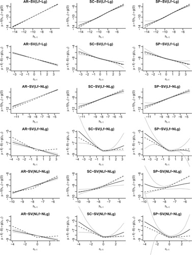
Table 2. For the three true leveraged SV models (Lf-Lg, Lf-NLg and NLf-NLg), a summary of the MSE and MAE of the log volatilities, $\{h_t{\}}_{t=1}^N$, obtained from fitting five different SV models. The averages and standard errors are multiplied by 100, and are based on 200 replicate series.

True model		Fitted models
		AR-SV	SC-SV(10)	SP-SV(10)	SC-SV(20)	SP-SV(20)
Lf-Lg
Average (s.e.)	MSE	38.0(0.2)	39.5(0.2)	39.6(0.2)	39.7(0.2)	40.3(0.3)
	MAE	48.5(0.1)	49.6(0.1)	49.6(0.1)	49.7(0.1)	50.0(0.2)
Rel. to AR-SV	MSE	100.0%	104.2%	104.3%	104.7%	106.1%
	MAE	100.0%	102.3%	102.3%	102.5%	103.1%
Lf-NLg		AR-SV	SC-SV(10)	SP-SV(10)	SC-SV(20)	SP-SV(20)
Average (s.e.)	MSE	35.3(0.2)	30.9(0.1)	31.2(0.1)	31.0(0.1)	31.7(0.3)
	MAE	47.2(0.1)	44.3(0.1)	44.6(0.1)	44.4(0.1)	44.8(0.1)
Rel. to AR-SV	MSE	100.0%	87.5%	88.5%	87.9%	89.6%
	MAE	100.0%	93.9%	94.4%	94.2%	94.9%
NLf-NLg		AR-SV	SC-SV(10)	SP-SV(10)	SC-SV(20)	SP-SV(20)
Average (s.e.)	MSE	25.5(0.1)	21.8(0.1)	26.3(0.3)	22.0(0.1)	27.0(0.3)
	MAE	40.2(0.1)	37.4(0.1)	41.2(0.3)	37.6(0.1)	41.9(0.3)
Rel. to AR-SV	MSE	100.0%	85.5%	103.2%	86.4%	105.9%
	MAE	100.0%	93.0%	102.4%	93.6%	104.2%

Table 3. Predictive log likelihood of daily returns from November 1, 2010 to October 31, 2013 using six different SV models. (u) – unleveraged; (l) – leveraged. The results of the best performing model (those with the largest predictive log likelihood) are in bold face.

	AR-SV(u)	SC-SV (u)	SP-SV (u)	AR-SV(l)	SC-SV (l)	SP-SV (l)
S&P500	−3798.8	−3796.5	−3799.3	−3784.5	−3784.2	−3786.0
EQR	−4080.5	−4068.8	−4072.0	−4080.4	−4070.6	−4079.5
MSFT	−4103.6	−4100.7	−4100.8	−4102.6	−4099.4	−4103.1
JnJ	−3681.7	−3682.9	−3684.2	−3680.9	−3680.7	−3681.7

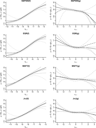
Figure 3. Fitted autoregressive function f and leverage function g for the daily returns of the S&P500, EQR, MSFT and JnJ. The solid lines show the posterior means and 95% credible bands of the fitted functions in the leveraged semiparametric models with shape constraints while the dashed lines represent the posterior means and 95% credible bands in the leveraged semiparametric models without shape constraints.