Small area prediction of quantiles for zero-inflated data and an informative sample design

Figures & data

Table 1. Comparison of MC bias and MC MSE for LIGPD predictors.

τ	Criterion	Predictor	$n_i=5$	$n_i=10$	$n_i=20$
0.25	MSE	SRS	0.0403	0.0229	0.0166
0.25	MSE	Inf	0.0316	0.0146	0.0077
0.25	Bias	SRS	−0.0954	−0.0935	−0.0965
0.25	Bias	Inf	−0.0166	−0.0145	−0.0174
0.50	MSE	SRS	0.0636	0.0453	0.0387
0.50	MSE	Inf	0.0349	0.0173	0.0095
0.50	Bias	SRS	−0.1740	−0.1720	−0.1756
0.50	Bias	Inf	−0.0322	−0.0301	−0.0338
0.75	MSE	SRS	0.1656	0.1446	0.1352
0.75	MSE	Inf	0.0546	0.0316	0.0204
0.75	Bias	SRS	−0.3442	−0.3472	−0.3508
0.75	Bias	Inf	−0.0654	−0.0686	−0.0725

Notes: SRS: predictors ignoring sampling weights. Inf: predictors that incorporate the modification for informative sampling defined in Section 3.1.

Figure 1. Black: predictors of quartiles and the median based on the zero-inflated quantile regression model. Top left: 25 percentile. Top right: median. Bottom: 75 percentile. Solid black line: predictors do not use sampling weights. Dashed black line: predictors incorporate the sampling weights through the preocedure of Section 3.1. Green and red: upper and lower endpoints of 95% prediction intervals.

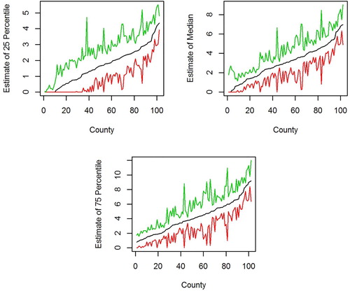
Figure 2. Comparison of predictors that incorporate the modification for informative sampling (x-axis) to predictors that do not use the sampling weights (y-axis). Top left: 25 percentiles. Top right: median. Bottom: 75 percentile.

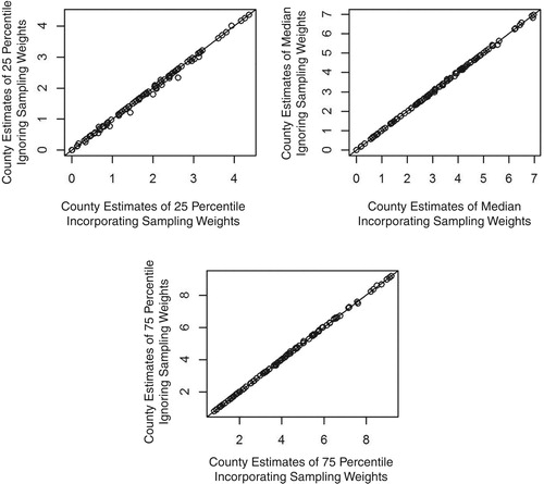
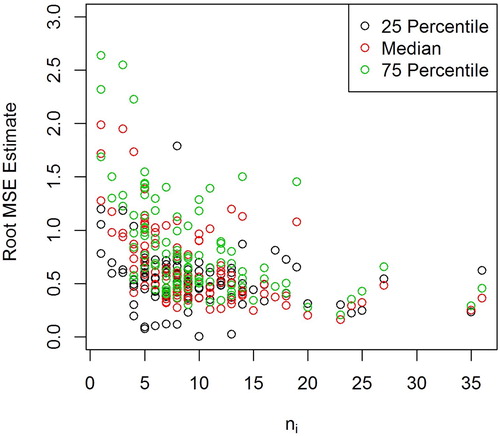
Figure 3. Estimated root mean squared errors plotted against county sample sizes. Estimated mean squared errors are defined in (32(32) ${\widehat{MSE}}_i\left(\tau \right)=\frac{1}{T}\sum _{t=1}^T\left({\hat{q}}_i^{\ast \left(t\right)}\right(\tau )-q_i^{\ast \left(t\right)}(\tau ){)}^2.$(32) ).