New extreme value theory for maxima of maxima

Figures & data

Figure 1. Simulated mixed sequences from normal and uniform distributions and their maxima (marked with black dots). In (a), the maximum is from the uniform distribution; in (b), the maximum is from $N(0,1)$.

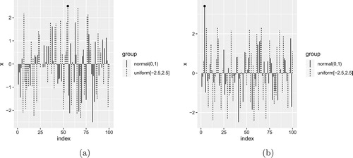
Figure 2. (a) Histogram of $M_n$ from $N(0,1)$ and $U[-2.2,2.2]$. (b) Histogram of $M_n$ from $N(0,1)$ and $U[-2.8,2.8]$.

Figure 3. Histograms of combinations of $M_n$ from $N(0,0.9)$ and $U[-2,2]$. (a) $n_1=100$, $n_2=200$. (b) $n_1=200$, $n_2=100$.

Figure 4. Histograms of $M_n$. (a) $N(0,1)$ and Fréchet combination. (b)–(d) Some combinations of Fréchet and Weibull.

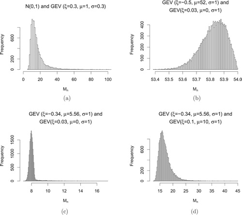
Figure 5. Histograms of $M_n$, with combinations of normal distribution and Weibull distribution.

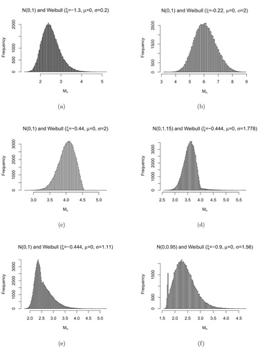
Figure 6. Density plots of the accelerated max-stable distributions with Weibull-Gumbel combinations. (a) ${\xi }_1=0$, ${\mu }_1=0.5$, ${\sigma }_1=1$, ${\xi }_2=-1$, ${\mu }_2=-1$, ${\sigma }_2=1$. (b) ${\xi }_1=0$, ${\mu }_1=0.5$, ${\sigma }_1=1$, ${\xi }_2=-1$, ${\mu }_2=0.5$, ${\sigma }_2=1$.

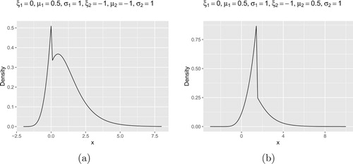
Figure 7. Density plots of the accelerated max-stable distributions with Weibull-Gumbel combinations. (a) ${\xi }_1=-1$, ${\mu }_1=-1$, ${\sigma }_1=1$, ${\xi }_2=0$, ${\mu }_2=0.5$, ${\sigma }_2=0.7$. (b) ${\xi }_1=-0.5$, ${\mu }_1=-2$, ${\sigma }_1=1$, ${\xi }_2=0$, ${\mu }_2=-1$, ${\sigma }_2=0.7$.

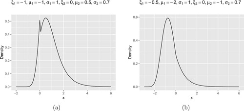
Figure 8. (a) Density plot of the accelerated max-stable distribution with Fréchet-Fréchet combinition. ${\xi }_1=0.5$, ${\mu }_1=0$, ${\sigma }_1=1$, ${\xi }_2=0.9$, ${\mu }_2=0$, ${\sigma }_2=1$. (b) Density plot of the accelerated max-stable distributions with Fréchet-Gumbel combinition. ${\xi }_1=0$, ${\mu }_1=0$, ${\sigma }_1=3$, ${\xi }_2=1$, ${\mu }_2=-3$, ${\sigma }_2=0.2$.

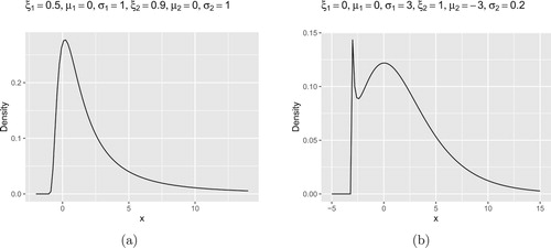
Figure 9. (a) Density plot of the accelerated max-stable distribution with Weibull-Fréchet combination. ${\xi }_1=-0.5$, ${\mu }_1=0$, ${\sigma }_1=1$, ${\xi }_2=0.3$, ${\mu }_2=-1$, ${\sigma }_2=0.1$. (b) Density plot of the accelerated max-stable distribution with Gumbel-Gumbel combinition. ${\xi }_1=0$, ${\mu }_1=0$, ${\sigma }_1=3$, ${\xi }_2=0$, ${\mu }_2=-3$, ${\sigma }_2=0.3$.

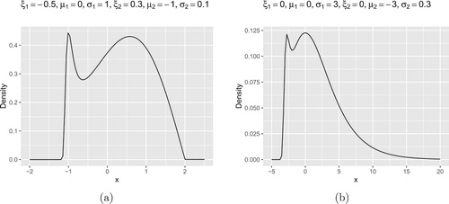
Table 1. The proportions of the simulated data based on the fitted accelerated max-stable distributions and GEV distributions that exceeds the 90th, 95th and 99th percentiles of the original data $Z_i$.

							90th		95th		99th
	${\xi }_1$	${\mu }_1$	${\sigma }_1$	${\xi }_2$	${\mu }_2$	${\sigma }_2$	AEVD	GEV	AEVD	GEV	AEVD	GEV
1	0.1	0	1	−0.1	0	1	0.1002	0.1071	0.0502	0.0540	0.0104	0.0094
							(0.005)	(0.006)	(0.004)	(0.004)	(0.002)	(0.002)
2	0.1	0	1	−0.2	2	1	0.0988	0.1191	0.0496	0.0688	0.0102	0.0140
							(0.005)	(0.006)	(0.004)	(0.006)	(0.002)	(0.003)
3	0	0	1	−0.2	2	1	0.1022	0.1094	0.0516	0.0555	0.0097	0.0088
							(0.009)	(0.008)	(0.007)	(0.006)	(0.003)	(0.003)
4	0	0	1	−0.1	0	1	0.1008	0.1039	0.0507	0.0525	0.0102	0.0096
							(0.007)	(0.008)	(0.006)	(0.006)	(0.003)	(0.003)
5	-0.1	0	1	−0.2	0	1	0.1007	0.1052	0.0502	0.0534	0.0103	0.0100
							(0.007)	(0.008)	(0.005)	(0.006)	(0.003)	(0.003)
6	-0.3	2	1	−0.15	0	1	0.1010	0.1024	0.0506	0.0514	0.0104	0.0098
							(0.008)	(0.008)	(0.006)	(0.006)	(0.002)	(0.003)
7	0	10	1	0.1	0	1	0.0997	0.1029	0.0505	0.0519	0.0104	0.0096
							(0.007)	(0.008)	(0.006)	(0.006)	(0.002)	(0.003)
8	0	30	1	0.05	0	1	0.0996	0.1033	0.0497	0.0520	0.0104	0.0098
							(0.008)	(0.008)	(0.005)	(0.006)	(0.002)	(0.003)
9	0.1	30	1	0.15	0	1	0.1002	0.1030	0.0507	0.0520	0.0106	0.0099
							(0.007)	(0.008)	(0.005)	(0.006)	(0.003)	(0.003)
10	0.05	20	1	0.08	0	1	0.0995	0.1025	0.0497	0.0517	0.0104	0.0098
							(0.007)	(0.008)	(0.006)	(0.006)	(0.003)	(0.003)
11	0	5	1	0	0	1	0.0996	0.1031	0.0502	0.0518	0.0104	0.0098
							(0.007)	(0.008)	(0.005)	(0.006)	(0.003)	(0.003)
12	0	2	1	0.2	0	1	0.1021	0.1077	0.0506	0.0548	0.0107	0.0095
							(0.007)	(0.009)	(0.005)	(0.007)	(0.003)	(0.003)

Notes: $\{Z_i{\}}_{i=1}^n$ is generated by taking the paired maxima of simulated sequences $\{X_i{\}}_{i=1}^n$ and $\{Y_i{\}}_{i=1}^n$ from two different GEV distributions. The standard deviations of the 100 repetitions are shown in the parentheses. The numbers in bold font are the ones that are closer to the theoretical values, i.e., 0.1, 0.05, and 0.01.

Figure 10. The histogram of the daily maxima of negative log returns of 330 stocks in the S&P 500 companies list.

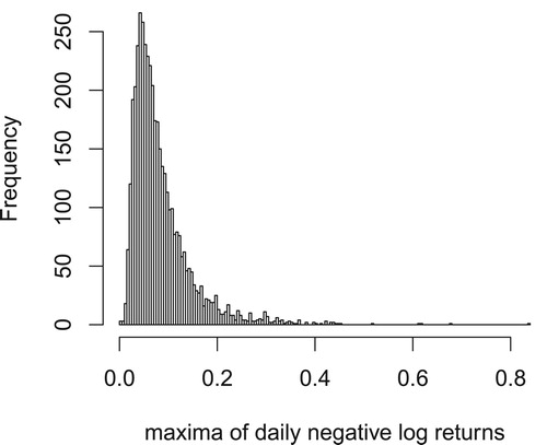
Table 2. The proportions of the simulated samples generated from the fitted distributions that exceed the 90th, 95th, and 99th sample percentiles of the maximal daily negative log returns.

	90th		95th		99th
	AMSD	GEV	AMSD	GEV	AMSD	GEV
Proportion	0.0961	0.0954	0.0475	0.0521	0.0115	0.0140

Note: The numbers in bold font are the ones that are closer to the theoretical values, i.e., 0.1, 0.05, and 0.01, respectively.