
Figures & data
Figure 1. The performance comparison of deep learning and machine learning.
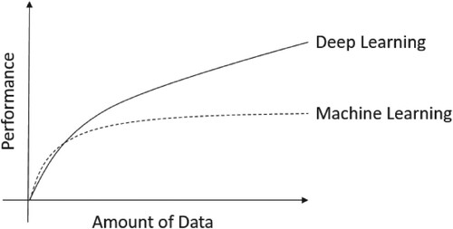
Figure 2. Illustration of GD iteration trajectory with learning rate 0.05.
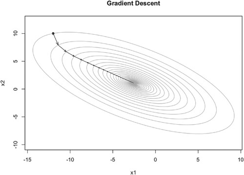
Figure 3. Illustration of GD iteration trajectory with learning rate 0.1.
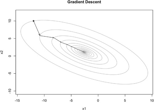
Figure 4. Illustration of GD iteration trajectory with learning rate 0.12.
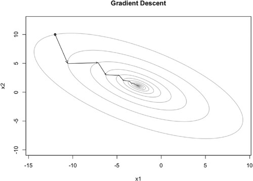
Figure 5. Illustration of OGD iteration trajectory.
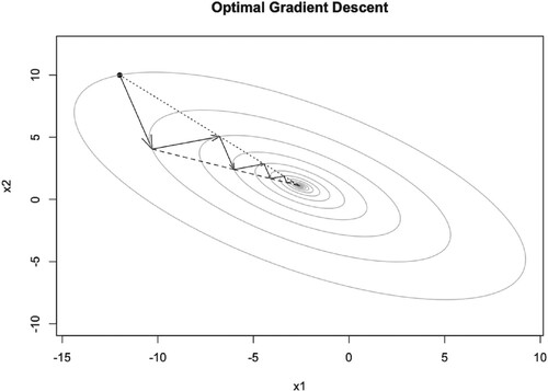
Figure 6. Illustration of PM iteration trajectory with and
.
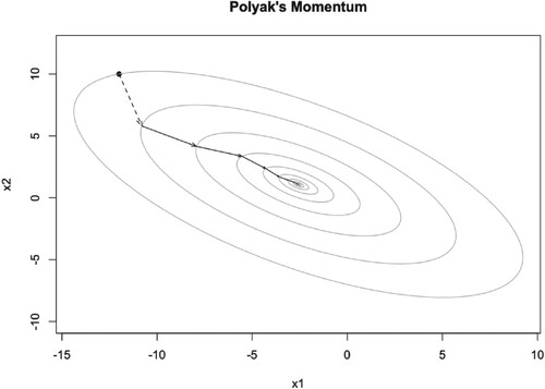
Figure 7. Illustration of PM iteration trajectory with and
.
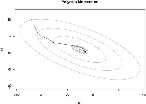
Figure 8. Illustration of PM iteration trajectory with and
.
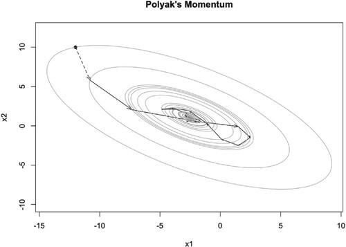
Table 1. Iteration steps of PM, NAG, and TAG algorithms with learning rate , while the steps of GD algorithm is 117.
Table 2. Iteration steps of PM, NAG, and TAG algorithms with learning rate , while the steps of GD algorithm is 54.
Table 3. Iteration steps of PM, NAG, and TAG algorithms with learning rate , while the steps of GD algorithm is 44.
Figure 9. Illustration of NAG iteration trajectory with and
.
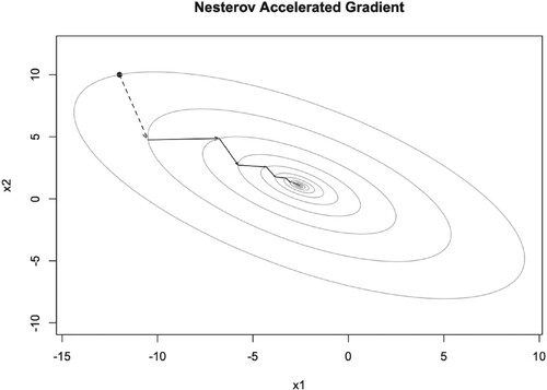
Figure 10. Illustration of NAG iteration trajectory with and
.
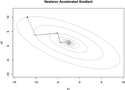
Figure 11. Illustration of NAG iteration trajectory with and
.
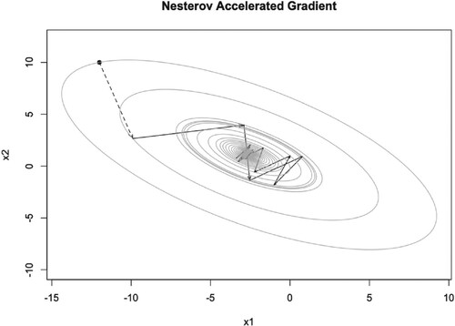
Figure 12. Illustration of TAG iteration trajectory for two-dimensional quadratic function with line search.
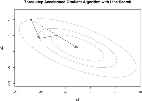
Figure 13. Illustration of TAG iteration trajectory with and
.

Figure 14. Illustration of TAG iteration trajectory with and
.

Figure 15. Illustration of TAG iteration trajectory with and
.
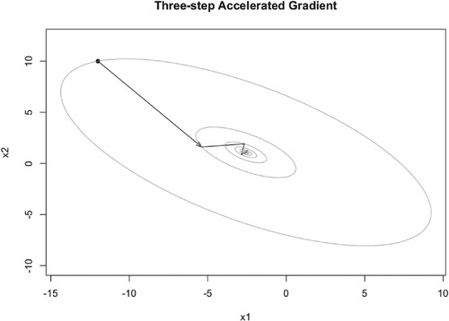
Figure 16. Illustration of TAG iteration trajectory with and
.
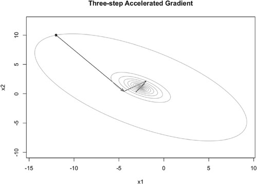
Table 4. Iteration steps and runtime (within parentheses) of 10-dimensional quadratic function.
Table 5. Iteration steps and runtime (within parentheses) of 100-dimensional quadratic function.
Table 6. Iteration steps and runtime (within parentheses) of 500-dimensional quadratic function.
Table 7. Iteration steps, runtime (within parentheses), and optimal μ with its range (within brackets) for 10-dimensional FLETCHCR function.
Table 8. Iteration steps, runtime (within parentheses), and optimal μ with its range (within brackets) for 100-dimensional FLETCHCR function.
Table 9. Iteration steps, runtime (within parentheses), and optimal μ with its range (within brackets) for 500-dimensional FLETCHCR function.
Figure 17. The scatter plot of spiral data.
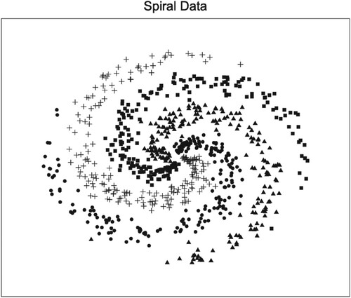
Figure 18. Feedforward neural network with 3 hidden layers.
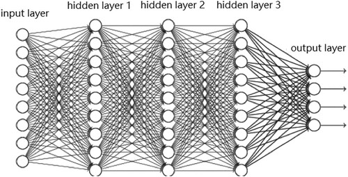
Figure 19. The scatter plot of iris petal.
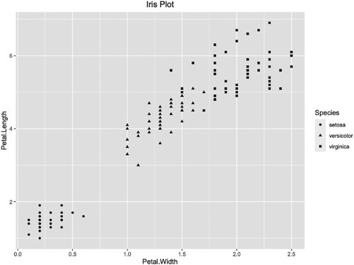
Figure 20. BPTAG algorithm training results of iris data set with and
.
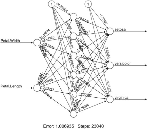
Table 10. Iteration steps and runtime (within parentheses) of BPPM, BPNAG, and BPTAG algorithms with learning rate for iris data set, while the steps and runtime of BPGD algorithm are 64822 and 17.88s respectively.
Table 11. Iteration steps and runtime (within parentheses) of BPPM, BPNAG, and BPTAG algorithms with learning rate for iris data set, while the steps and runtime of BPGD algorithm is 48849 and 11.77s respectively.
Table 12. Iteration steps and runtime (within parentheses) of BPPM, BPNAG, and BPTAG algorithms with learning rate for iris data set, while the steps and runtime of BPGD algorithm is 33503 and 8.09s respectively.
Table 13. Training accuracy of BPPM, BPNAG, and BPTAG algorithms with learning rate for spiral data set, while the accuracy of BPGD algorithm is 0.8775.
Table 14. Training accuracy of BPPM, BPNAG, and BPTAG algorithms with learning rate for spiral data set, while the accuracy of BPGD algorithm is 0.8950.
Table 15. Training accuracy of BPPM, BPNAG, and BPTAG algorithms with learning rate for spiral data set, while the accuracy of BPGD algorithm is 0.8975.
Figure 21. BPTASG algorithm training results of iris data set with and
.
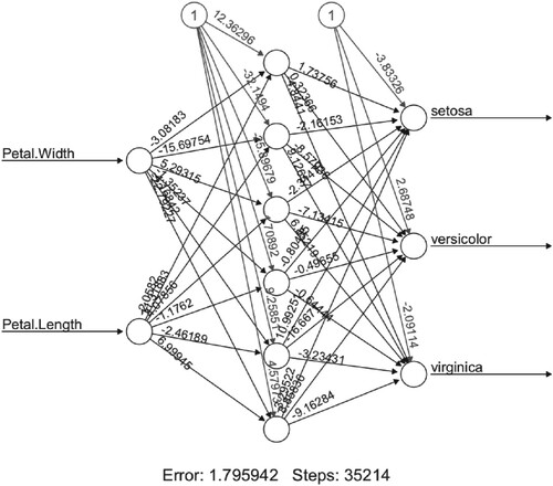
Table 16. Iteration steps and runtime (within parentheses) of BPPMSGD, BPNASG, and BPTASG algorithms with learning rate for iris data set, while the steps and runtime of BPSGD algorithm is 123859 and 22.13s respectively.
Table 17. Training accuracy of BPPMSGD, BPNASG, and BPTASG algorithms with learning rate for spiral data set, while the accuracy of BPSGD algorithm is 0.8887.