Mathematical model of malaria transmission dynamics with distributed delay and a wide class of nonlinear incidence rates

Figures & data

Figure 1. The dashed arrows indicate the direction of the infection and the solid arrows represent the transition from one class to another.

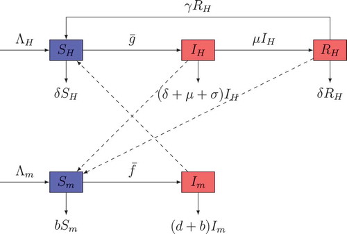
Figure 2. Density of infected mosquitoes and infected humans when, $\gamma =0.4$, $\delta =0.0187$, $\alpha =0.3$, $d=0.1$, $\mu =0.018$, $b=0.11$, ${\mathrm{\Lambda }}_H=0.29$, ${\mathrm{\Lambda }}_m=0.2$, $\beta =0.021$, $\sigma =0.011$ and $\tau =0.34$ and $\tau =1.34$ respectively for the sub-figures (a) and (b).

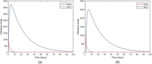
Figure 3. Periodic solutions with delay $\tau =0.1$ and $\gamma =0.01$, $\delta =0.011$, $\alpha =0.19$, $d=0.22$, $\mu =0.022$, $b=0.11$, ${\mathrm{\Lambda }}_H=0.4$, ${\mathrm{\Lambda }}_m=0.29$, $\beta =0.29$, $\sigma =0.011$.

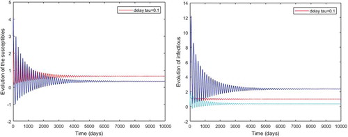
Figure 4. Periodic solutions with a length incubation period $\tau =1.6$ and $\gamma =0.01$, $\delta =0.011$, $\alpha =0.19$, $d=0.22$, $\mu =0.022$, $b=0.11$, ${\mathrm{\Lambda }}_H=0.4$, ${\mathrm{\Lambda }}_m=0.29$, $\beta =0.29$, $\sigma =0.011$.

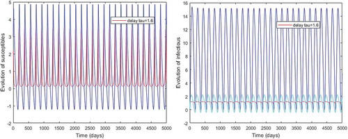
Figure 5. Density of infected mosquitoes versus susceptible mosquitoes; and susceptible mosquitoes versus infected mosquitoes when $\tau =0.1$ and $\gamma =0.01$, $\delta =0.011$, $\alpha =0.19$, $d=0.22$, $\mu =0.022$, $b=0.11$, ${\mathrm{\Lambda }}_H=0.4$, ${\mathrm{\Lambda }}_m=0.29$, $\beta =0.29$, $\sigma =0.011$.

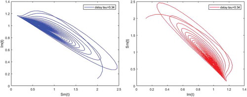
Figure 6. Density of infected humans versus susceptible humans; and susceptible humans versus partially immune individuals when $\tau =0.1$ and $\gamma =0.01$, $\delta =0.011$, $\alpha =0.19$, $d=0.22$, $\mu =0.022$, $b=0.11$, ${\mathrm{\Lambda }}_H=0.4$, ${\mathrm{\Lambda }}_m=0.29$, $\beta =0.29$, $\sigma =0.011$.

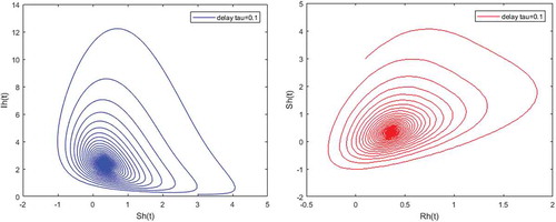
Figure 7. Density of partially immune individuals versus susceptible; and infected humans versus partially immune individuals when $\tau =0.34$ and $\gamma =0.01$, $\delta =0.011$, $\alpha =0.19$, $d=0.22$, $\mu =0.022$, $b=0.11$, ${\mathrm{\Lambda }}_H=0.4$, ${\mathrm{\Lambda }}_m=0.29$, $\beta =0.29$, $\sigma =0.011$.

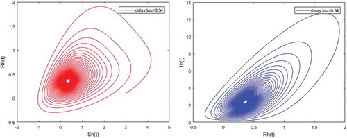
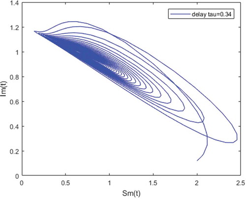
Figure 8. Limit cycles appearance when $\tau =1.34$ and $\gamma =0.01$, $\delta =0.011$, $\alpha =0.19$, $d=0.22$, $\mu =0.022$, $b=0.11$, ${\mathrm{\Lambda }}_H=0.4$, ${\mathrm{\Lambda }}_m=0.29$, $\beta =0.29$, $\sigma =0.011$.