Search in:

Arab Journal of Basic and Applied Sciences Volume 26, 2019 - Issue 1

Submit an article Journal homepage

Open access

782

Views

CrossRef citations to date

Altmetric

Original Articles

A comparative study of analytical solutions of space-time fractional hyperbolic-like equations with two reliable methods

Brajesh Kumar SinghDepartment of Mathematics, School of Physical and Decision Sciences, Babasaheb Bhimrao Ambedkar University, Lucknow, IndiaCorrespondence[email protected]

http://orcid.org/0000-0003-0121-8274

Mukesh GuptaDepartment of Mathematics, School of Physical and Decision Sciences, Babasaheb Bhimrao Ambedkar University, Lucknow, India

http://orcid.org/0000-0002-2070-6911

Pages 41-57 | Received 18 Apr 2018, Accepted 13 Oct 2018, Published online: 21 Mar 2019

Cite this article
https://doi.org/10.1080/25765299.2018.1538067
CrossMark

Full Article
Figures & data
References
Citations
Metrics
Licensing
Reprints & Permissions
View PDF PDF View EPUB EPUB

Figures & data

Figure 3. The solution behavior of Example 3.3 obtained by using NIPDTM. (a) Comparison of different order solutions with exact solutions for α = β = 2, x = y = z = 1, t ≤ 16. (b) Absolute errors in different order solutions for α = β = 2, x = y = z = 1, t ≤ 1. (c) Absolute errors in 5th order solutions for α = β = 2 y = z = 1, t ≤ 1. (d) Absolute errors in 7th order solutions for α = β = 2, y = z = 1, t ≤ 1.

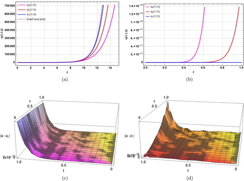
Table 1. Comparison of absolute errors for α = β = 2 at different time levels $t \leq 1$ .

Display Table

Table 2. mth order approximate solutions $S_{m} (m = 5, 7)$ of example 3.1 for $α = β = 1.5$ at different time levels $t \leq 1$ .

Display Table

Figure 1. The solution behavior of Example 3.1 obtained by using NIPDTM. (a) Absolute error in 5th order solution for α = β = 2. (b) Absolute error in 7th order solution α = β = 2. (c) Different order solutions for α = β = 2 for large time interval. (d) Sixth order solution for different values of α, β. (e) Eighth order solution for α = β = 2 with x = 1, t ∈ (0, 1). (f) Eighth order solution for α = 1.75, β = 1.85 with x = 1, t ∈ (0, 1).

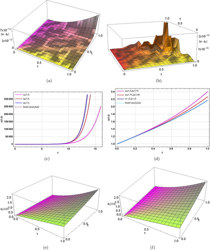
Figure 2. The solution behavior of Example 3.2 obtained by using NIPDTM. (a) Comparison of different order solutions with exact solutions for α = β = 2, x = y = 1, t ≤ 16. (b) Absolute errors in different order solutions for α = β = 2, x = y = 1, t ≤ 1. (c) Absolute errors in 5th order solutions for α = β = 2, y = 1, t ≤ 1. (d) Absolute errors in 7th order solutions for α = β = 2, y = 1, t ≤ 1. (e) Seventh order solution behavior for α = 1.25, β = 1.5 at t = 1. (f) Seventh order solution behavior for α = 1.5, β = 1.75 at t = 1. (g) Seventh order solution behavior for α = 2, β = 2 at t = 1. (h) Plots of seventh order solutions for different α, β, x = y = 1.

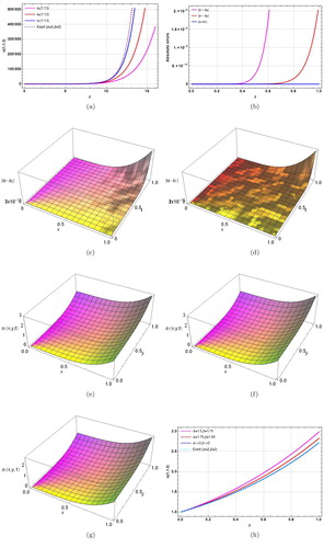
Table 3. Comparison of absolute errors in of example 3.2 for $α = β = 2$ at different time levels $t \leq 1$ .

Display Table

Table 4. mth order approximate solutions $S_{m} (m = 5, 7)$ of example 3.2 for $α = β = 1.5$ at different time levels $t \leq 1$ .

Display Table

Table 5. Comparison of absolute errors in of example 3.3 for $α = β = 2$ at different time levels $t \leq 1$ .

Display Table

Table 6. mth order approximate solutions $S_{m} (m = 5, 7)$ of example 3.3 for z = 0.2, $α = β = 1.5$ at different time levels $t \leq 1$ .

Display Table

Related Research Data

Exact solutions of fractional heat-like and wave-like equations with variable coefficients

Source: Emerald

Fractal behavior in trapping and reaction: A random walk study

Source: Springer Science and Business Media LLC

Fractional control of heat diffusion systems

Source: Springer Science and Business Media LLC

Analysis of a time fractional wave-like equation with the homotopy analysis method

Source: Elsevier BV

Solution for a Fractional Diffusion-Wave Equation Defined in a Bounded Domain

Source: Springer Science and Business Media LLC

Extended Fractional Reduced Differential Transform for Solving Fractional Partial Differential Equations with Proportional Delay

Source: Springer Science and Business Media LLC

Reduced differential transform method for solving parabolic-like and hyperbolic-like equations

Source: Springer Science and Business Media LLC

He's homotopy perturbation method for solving heat-like and wave-like equations with variable coefficients

Source: Elsevier BV

Fractals and fractional calculus in continuum mechanics

Source: Springer Vienna

Homotopy perturbation technique

Source: Elsevier BV

Space-fractional advection-dispersion equations by the Kansa method

Source: Elsevier BV

A modified homotopy analysis method for solution of fractional wave equations

Source: SAGE Publications

Method of approximate particular solutions for constant- and variable-order fractional diffusion models

Source: Elsevier BV

Fractional Relaxation-Oscillation and Fractional Diffusion-Wave Phenomena

Source: Elsevier BV

New Fractional Derivatives with Nonlocal and Non-Singular Kernel: Theory and Application to Heat Transfer Model

Source: National Library of Serbia

Modification of the pattern informatics method for forecasting large earthquake events using complex eigenfactors

Source: arXiv

Mixture of a New Integral Transform and Homotopy Perturbation Method for Solving Nonlinear Partial Differential Equations

Source: Scientific Research Publishing, Inc.

A General Iteration Formula of VIM for Fractional Heat- and Wave-Like Equations

Source: Hindawi Publishing Corporation

Boundary particle method for Laplace transformed time fractional diffusion equations

Source: Elsevier BV

Variational iteration method for fractional heat- and wave-like equations

Source: Elsevier BV

Approximate analytic solution of fractional heat-like and wave-like equations with variable coefficients using the differential transforms method

Source: Springer Nature

(N+1)-dimensional fractional reduced differential transform method for fractional order partial differential equations

Source: Elsevier BV

Fractional Dynamics and Control

Source: Springer New York

Non-homogeneous elastic waves in soils: Notes on the vector decomposition technique

Source: Elsevier BV

Semi- analytic numerical method for solution of time-space fractional heat and wave type equations with variable coefficients

Source: DE GRUYTER

Fractional-order diffusion-wave equation

Source: Springer Science and Business Media LLC

Beyond Adomian method: The variational iteration method for solving heat-like and wave-like equations with variable coefficients

Source: Elsevier BV

Exact solutions of time fractional heat-like and wave-like equations with variable coefficients

Source: VINCA Institute of Nuclear Sciences

Analytical approximate solution for fractional heat-like and wave-like equations with variable coefficients using the decomposition method

Source: Elsevier BV

Front propagation in anomalous diffusive media governed by time-fractional diffusion

Source: Elsevier BV

Fractional Vector Calculus and Fractional Maxwell's Equations

Source: arXiv

Multidimensional solutions of time-fractional diffusion-wave equations

Source: The Royal Society

Homotopy perturbation method for two dimensional time-fractional wave equation

Source: Elsevier BV

SOLVING FRACTIONAL DIFFUSION AND WAVE EQUATIONS BY MODIFIED HOMOTOPY PERTURBATION METHOD

Source: Elsevier BV

Linking provided by

Related research

People also read lists articles that other readers of this article have read.

Recommended articles lists articles that we recommend and is powered by our AI driven recommendation engine.

Cited by lists all citing articles based on Crossref citations.
Articles with the Crossref icon will open in a new tab.

People also read
Recommended articles
Cited by

To cite this article:

Reference style: APA Chicago Harvard

Citation copied to clipboard

Reference styles above use APA (6th edition), Chicago (16th edition) & Harvard (10th edition)

Download citation

Download a citation file in RIS format that can be imported by citation management software including EndNote, ProCite, RefWorks and Reference Manager.

Choose format: RIS BibTex RefWorks Direct Export

Choose options: Citation Citation & abstract Citation & references

A comparative study of analytical solutions of space-time fractional hyperbolic-like equations with two reliable methods

Table 1. Comparison of absolute errors for α = β = 2 at different time levels $t \leq 1$ .

Table 2. mth order approximate solutions $S_{m} (m = 5, 7)$ of example 3.1 for $α = β = 1.5$ at different time levels $t \leq 1$ .

Table 3. Comparison of absolute errors in of example 3.2 for $α = β = 2$ at different time levels $t \leq 1$ .

Table 4. mth order approximate solutions $S_{m} (m = 5, 7)$ of example 3.2 for $α = β = 1.5$ at different time levels $t \leq 1$ .

Table 5. Comparison of absolute errors in of example 3.3 for $α = β = 2$ at different time levels $t \leq 1$ .

Table 6. mth order approximate solutions $S_{m} (m = 5, 7)$ of example 3.3 for z = 0.2, $α = β = 1.5$ at different time levels $t \leq 1$ .

Related Research Data

Information for

Open access

Opportunities

Help and information

Your download is now in progress and you may close this window

Login or register to access this feature

A comparative study of analytical solutions of space-time fractional hyperbolic-like equations with two reliable methods

Figures & data

Table 1. Comparison of absolute errors for α = β = 2 at different time levels t≤1.

Table 2. mth order approximate solutions Sm (m=5,7) of example 3.1 for α=β=1.5 at different time levels t≤1.

Table 3. Comparison of absolute errors in of example 3.2 for α=β=2 at different time levels t≤1.

Table 4. mth order approximate solutions Sm (m=5,7) of example 3.2 for α=β=1.5 at different time levels t≤1.

Table 5. Comparison of absolute errors in of example 3.3 for α=β=2 at different time levels t≤1.

Table 6. mth order approximate solutions Sm (m=5,7) of example 3.3 for z = 0.2, α=β=1.5 at different time levels t≤1.

Related Research Data

Related research

To cite this article:

Download citation

Information for

Open access

Opportunities

Help and information

Keep up to date

Table 1. Comparison of absolute errors for α = β = 2 at different time levels $t \leq 1$ .

Table 2. mth order approximate solutions $S_{m} (m = 5, 7)$ of example 3.1 for $α = β = 1.5$ at different time levels $t \leq 1$ .

Table 3. Comparison of absolute errors in of example 3.2 for $α = β = 2$ at different time levels $t \leq 1$ .

Table 4. mth order approximate solutions $S_{m} (m = 5, 7)$ of example 3.2 for $α = β = 1.5$ at different time levels $t \leq 1$ .

Table 5. Comparison of absolute errors in of example 3.3 for $α = β = 2$ at different time levels $t \leq 1$ .

Table 6. mth order approximate solutions $S_{m} (m = 5, 7)$ of example 3.3 for z = 0.2, $α = β = 1.5$ at different time levels $t \leq 1$ .