Mathematical modelling for a fabrication–inventory problem with scrap, an acceptable stock-out level, stochastic failures and a multi-shipment policy

Figures & data

Figure 1. The on-hand inventory/backlog level at time t in the proposed system with a breakdown happening in t₄′.

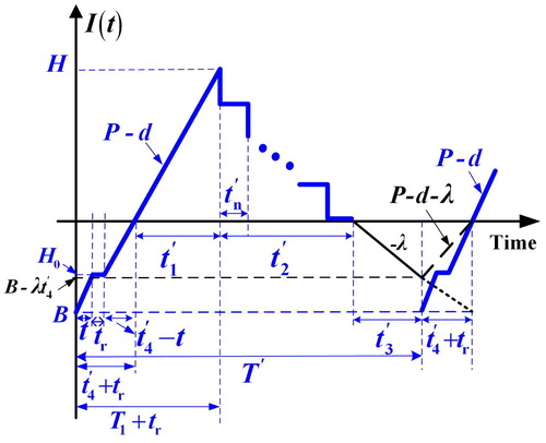
Figure 2. The on-hand scrap level at time t in the proposed system with a breakdown happening in t₄′.

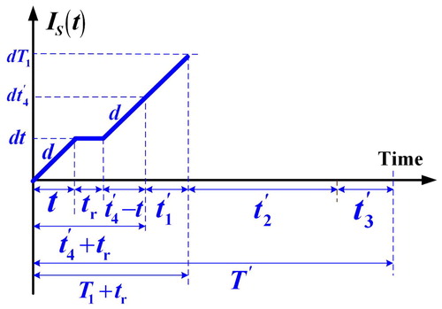
Figure 3. The on-hand finished product level in distribution time t₂′ in the proposed system with a breakdown happening in t₄′.

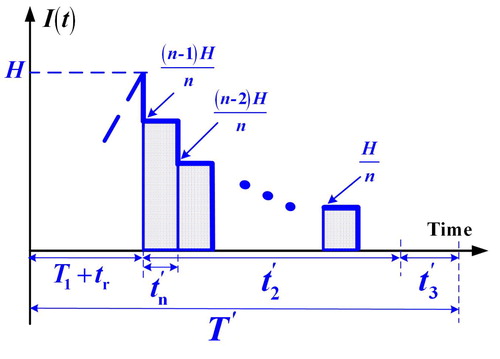
Figure 4. The on-hand inventory/backlog level at time t in the proposed system with a breakdown happening in the period of [t₄′, T₁].

Figure 5. The on-hand scrap level at time t in the proposed system with a breakdown happening in the period of [t₄′, T₁].

Figure 6. The on-hand inventory/backlog level at time t in the proposed system with no breakdown happening in uptime.

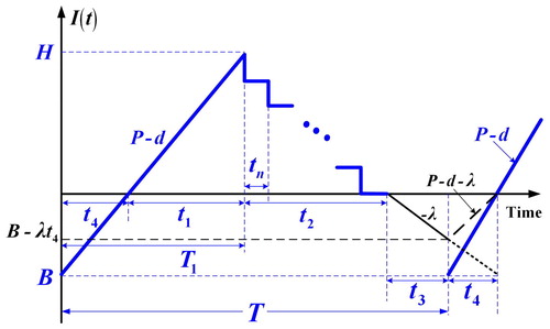
Table 1. Step-by-step computation results for finding T₁* (based on β = 0.5).

Step no.	e^–βT1U	T1U	E[TCU(T1U)]	e^–βT1L	T1L	E[TCU(T1L)]
1	0	0.604	$11,369.58	1	0.421	$11,311.50
2	0.740	0.471	$11,300.52	0.810	0.458	$11,300.80
3	0.790	0.462	$11,300.54	0.795	0.461	$11,300.59
4	0.794	0.461	$11,300.58	0.794	0.461	$11,300.58

Figure 7. The contributed percentages of each relevant cost components in E[TCU(T₁*)].

Figure 8. Impact of random scrap rate x on E[TCU(T₁*)].

Figure 9. Effect of variations in mean-time-to-failure (MTTF) 1/β on E[TCU(T₁*)].

Figure 10. Impact of random scrap rate x on T₁*.

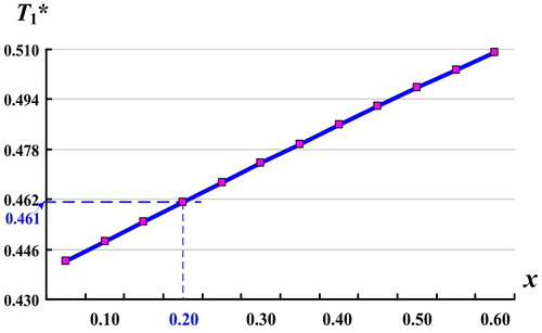
Figure 11. Effect of variations in T on E[TCU(T₁)].

Table 2. Effects of various service-level percentages on diverse system parameters/costs.

Service level (1 – α)%	Maximal stock holding level H	Maximal backlogging level B	Annual holding cost	Annual backordering cost	E[TCU(T1*)]	Percentage increase in E[TCU(T1*)]
100%	3509	0	$1,255	$0	$11,737	7.99
95%	3495	180	$1,197	$0	$11,620	6.91
90%	3472	378	$1,140	$2	$11,507	5.88
85%	3439	594	$1,084	$4	$11,401	4.89
80%	3391	830	$1,031	$8	$11,301	3.97
75%	3327	1085	$980	$14	$11,208	3.12
70%	3242	1359	$931	$20	$11,124	2.35
65%	3133	1648	$886	$29	$11,050	1.67
60%	2997	1950	$845	$39	$10,987	1.09
55%	2831	2257	$808	$51	$10,937	0.62
50%	2635	2563	$777	$64	$10,899	0.28
45%	2410	2858	$751	$79	$10,876	0.07
39%	2108	3184	$729	$97	$10,869	–

Figure 13. Impact of number of deliveries per cycle n on T₁*.

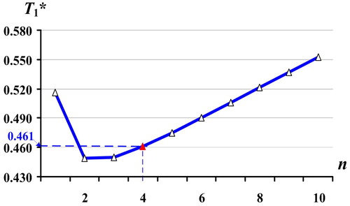
Figure 14. Effect of variations in service level constraint (1 – α) on E[TCU(T₁)].

Figure 15. Joint impacts of service-level constraint (1 – α) and 1/β on E[TCU(T₁*)].

Figure A-1. The on-hand scrap level at time t in the proposed system with no breakdown happening in uptime.

Figure 12. Impact of number of deliveries per cycle n on E[TCU(T₁*)].

Figure A-2. The on-hand finished product level in distribution time t₂′ in the proposed system with no breakdown happening in uptime.

Table B-1. Results of convexity test for E[TCU(T₁)] by using extra values of β.

β	T1U	Equation (30)*(30) $$\frac{2\left(z_1+\frac{n{K}_1}{P}+w_1+w_3{e}^{-\beta T_1}+\frac{w_5}{n}+\frac{w_7{e}^{-\beta T_1}}{n}\right)+z_0\left(1-e^{-\beta T_1}\right)}{\left(\begin{array}{c}-T_1{}^2{\beta }^2{w}_2{e}^{-\beta T_1}-T_1{\beta }^2{w}_3{e}^{-\beta T_1}-2\beta w_3{e}^{-\beta T_1}-T_1{}^2{\beta }^2{s}^2{w}_4{e}^{-\beta T_{1}s}-\frac{T_1{}^2{\beta }^2{w}_6{e}^{-\beta T_1}}{n}\\ -\frac{T_1{\beta }^2{w}_7{e}^{-\beta T_1}}{n}-\frac{2\beta w_7{e}^{-\beta T_1}}{n}-T_1\beta e^{-\beta T_1}{z}_0-T_1{}^2\beta e^{-\beta T_1}\left(\frac{h_3\lambda g}{P}\right)\end{array}\right)}>T_1>0$$(30)	T1L	z(T1L)**
5.00	0.560	3.516	0.259	1.101
4.00	0.561	2.810	0.286	1.207
3.00	0.563	2.398	0.317	1.358
2.00	0.567	2.276	0.354	1.619
1.00	0.580	2.687	0.397	2.270
0.50	0.604	3.602	0.421	3.224
:	:	:	:	:
0.01	1.778	11.790	0.447	7.450

* Denotes the computation result from the left-hand side of Equation (30)(30) $$\frac{2\left(z_1+\frac{n{K}_1}{P}+w_1+w_3{e}^{-\beta T_1}+\frac{w_5}{n}+\frac{w_7{e}^{-\beta T_1}}{n}\right)+z_0\left(1-e^{-\beta T_1}\right)}{\left(\begin{array}{c}-T_1{}^2{\beta }^2{w}_2{e}^{-\beta T_1}-T_1{\beta }^2{w}_3{e}^{-\beta T_1}-2\beta w_3{e}^{-\beta T_1}-T_1{}^2{\beta }^2{s}^2{w}_4{e}^{-\beta T_{1}s}-\frac{T_1{}^2{\beta }^2{w}_6{e}^{-\beta T_1}}{n}\\ -\frac{T_1{\beta }^2{w}_7{e}^{-\beta T_1}}{n}-\frac{2\beta w_7{e}^{-\beta T_1}}{n}-T_1\beta e^{-\beta T_1}{z}_0-T_1{}^2\beta e^{-\beta T_1}\left(\frac{h_3\lambda g}{P}\right)\end{array}\right)}>T_1>0$$(30) with T_1U.

** Stands for the computation result from the left-hand side of Equation (30)(30) $$\frac{2\left(z_1+\frac{n{K}_1}{P}+w_1+w_3{e}^{-\beta T_1}+\frac{w_5}{n}+\frac{w_7{e}^{-\beta T_1}}{n}\right)+z_0\left(1-e^{-\beta T_1}\right)}{\left(\begin{array}{c}-T_1{}^2{\beta }^2{w}_2{e}^{-\beta T_1}-T_1{\beta }^2{w}_3{e}^{-\beta T_1}-2\beta w_3{e}^{-\beta T_1}-T_1{}^2{\beta }^2{s}^2{w}_4{e}^{-\beta T_{1}s}-\frac{T_1{}^2{\beta }^2{w}_6{e}^{-\beta T_1}}{n}\\ -\frac{T_1{\beta }^2{w}_7{e}^{-\beta T_1}}{n}-\frac{2\beta w_7{e}^{-\beta T_1}}{n}-T_1\beta e^{-\beta T_1}{z}_0-T_1{}^2\beta e^{-\beta T_1}\left(\frac{h_3\lambda g}{P}\right)\end{array}\right)}>T_1>0$$(30) with T_1L.