A fractional-order generalized Richards growth model and its implementation to COVID-19 data

Figures & data

Figure 1. The cumulative number of cases C(t) for the GRM with different values of parameters.

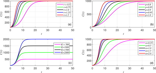
Figure 2. The corresponding daily new cases $C\prime (t)$ of Figure 1.

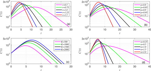
Figure 3. The cumulative number of cases C(t) obtained by the Caputo fractional-order generalized Richards model (left-panel) and the Atangana-Baleanu in the Caputo sense (ABC) fractional-order generalized Richards model (right-panel) with parameter values (a,b) $r=p=a=1,K=1000;$ (c,d) $r=0.1,p=a=1,K=1000;$ (e,f) $r=1,p=0.5,a=1,K=1000;$ and (g,h) $r=1,p=1,a=2,K=1000.$ The arrow shows increasing values of $\alpha =0.6,0.7,0.8,0.9,$ and 1.0.

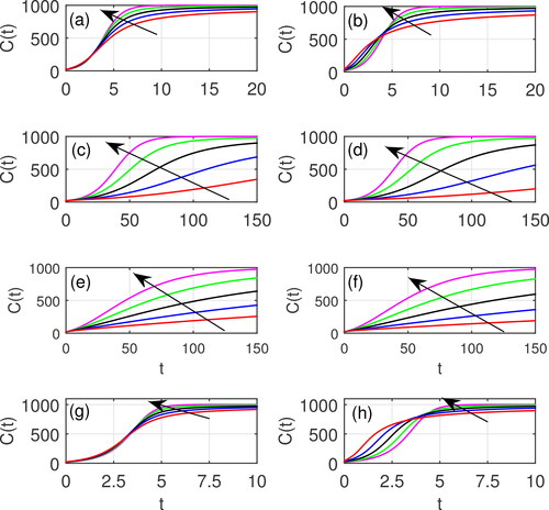
Figure 4. The corresponding daily new cases $C\prime (t)$ obtained by the Caputo fractional-order generalized Richards model (left-panel) and the Atangana-Baleanu in the Caputo sense (ABC) fractional-order generalized Richards model (right-panel) with parameter values (a,b) $r=p=a=1,K=1000;$ (c,d) $r=0.1,p=a=1,K=1000;$ (e,f) $r=1,p=0.5,a=1,K=1000;$ and (g,h) $r=1,p=1,a=2,K=1000.$ The arrow shows increasing values of $\alpha =0.6,0.7,0.8,0.9,$ and 1.0.

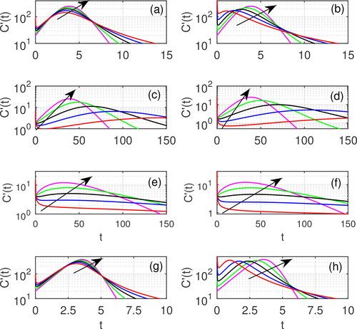
Figure 5. Cumulative number of COVID-19 cases (left-panel) and daily new cases of COVID-19 (right-panel) in East Java Province, Indonesia.

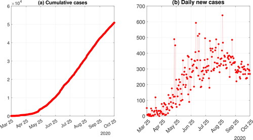
Figure 6. (a–f) Numerical solutions of the fitted GCFRM (3)(3) $${}^C{\mathcal{D}}_t^{\alpha }C(t)=\mathit{\text{rC}}{(t)}^p\left(1-{\left(\frac{C(t)}{K}\right)}^a\right),$$(3) compared to the confirmed COVID-19 data from east java. In the left panel, the fitted curves C(t) of the GCFRM (3)(3) $${}^C{\mathcal{D}}_t^{\alpha }C(t)=\mathit{\text{rC}}{(t)}^p\left(1-{\left(\frac{C(t)}{K}\right)}^a\right),$$(3) using three different data periods: namely (a) March 25 – May 24, 2020 (61 d), (c) march 25 – Jul 24, 2020 (122 d) and (e) march 25 – Oct 21, 2020 (211 d), are compared to the cumulative confirmed cases; while the right panels show the comparison between the corresponding fitted $C\prime (t)$ which are calculated numerically and the confirmed new daily cases.

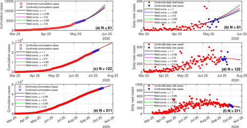
Figure 7. (a–f) Numerical solutions of the fitted GABCFRM (7)(7) $${}^{\mathit{\text{ABC}}}{\mathcal{D}}_t^{\alpha }C(t)=\mathit{\text{rC}}{(t)}^p\left(1-{\left(\frac{C(t)}{K}\right)}^a\right).$$(7) compared to the confirmed COVID-19 data from east java. In the left panel, the fitted curves C(t) of the GABCFRM (7)(7) $${}^{\mathit{\text{ABC}}}{\mathcal{D}}_t^{\alpha }C(t)=\mathit{\text{rC}}{(t)}^p\left(1-{\left(\frac{C(t)}{K}\right)}^a\right).$$(7) using three different data periods: namely (a) March 25 – May 24, 2020 (61 d), (c) march 25 – Jul 24, 2020 (122 d) and (e) march 25 – Oct 21, 2020 (211 d), are compared to the cumulative confirmed cases; while the right panels show the comparison between the corresponding fitted $C\prime (t)$ which are calculated numerically and the confirmed new daily cases.

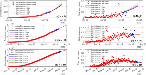
Table 1. Estimated value of parameter based on the GCFRM (3)(3) $${}^C{\mathcal{D}}_t^{\alpha }C(t)=\mathit{\text{rC}}{(t)}^p\left(1-{\left(\frac{C(t)}{K}\right)}^a\right),$$(3) for different value of α. Notice that α = 1 corresponds to the first order GRM (1)(1) $$\frac{\mathit{\text{dC}}(t)}{\mathit{\text{dt}}}=C\prime (t)=\widehat{r} C{(t)}^p\left(1-{\left(\frac{C(t)}{K}\right)}^a\right),$$(1) .

Number of Data	Parameter	α = 1	$\alpha =0.95$	$\alpha =0.9$	$\alpha =0.85$	$\alpha =0.8$
61	r	0.3487	0.1737	0.2092	0.2165	0.1952
	p	0.9458	0.9115	0.8634	0.8790	0.9718
	K	439,254	483,057	498,267	498,550	484,579
	a	0.0801	0.2275	0.9956	0.9971	0.1840
122	r	0.2260	0.1575	0.1652	0.1732	0.1821
	p	0.9525	0.9415	0.9526	0.9659	0.9789
	K	48,508	50,339	53,315	56,782	60,623
	a	0.2206	0.2931	0.2980	0.2940	0.2900
211	r	0.3891	0.2723	0.2710	0.2708	0.2721
	p	0.9072	0.9280	0.9405	0.9518	0.9618
	K	76,643	80,878	85,443	90,488	96,097
	a	0.1387	0.1282	0.1376	0.1486	0.1619

Table 2. Estimated value of parameter based on the GABCFRM (7)(7) $${}^{\mathit{\text{ABC}}}{\mathcal{D}}_t^{\alpha }C(t)=\mathit{\text{rC}}{(t)}^p\left(1-{\left(\frac{C(t)}{K}\right)}^a\right).$$(7) for different value of α. Notice that α = 1 corresponds to the first order GRM (1)(1) $$\frac{\mathit{\text{dC}}(t)}{\mathit{\text{dt}}}=C\prime (t)=\widehat{r} C{(t)}^p\left(1-{\left(\frac{C(t)}{K}\right)}^a\right),$$(1) .

Number of Data	Parameter	α = 1	$\alpha =0.95$	$\alpha =0.9$	$\alpha =0.85$	$\alpha =0.8$
61	r	0.3487	0.1739	0.1851	0.2159	0.1918
	p	0.9458	0.9151	0.9507	0.8861	0.9828
	K	439,254	478,176	452,523	499,644	442,946
	a	0.0801	0.2225	0.1685	0.9999	0.1883
122	r	0.2260	0.1580	0.1653	0.1733	0.1816
	p	0.9525	0.9424	0.9569	0.9698	0.9834
	K	48,508	50,261	53,296	56,581	60,344
	a	0.2206	0.2969	0.2983	0.3053	0.3103
211	r	0.3891	0.2726	0.2567	0.2692	0.2671
	p	0.9072	0.9297	0.9316	0.9579	0.9696
	K	76,643	80,839	85,168	90,379	95,977
	a	0.1387	0.1288	0.1697	0.1509	0.1685

Table 3. Coefficient of determination for the calibration of cumulative number of cases.

	GCFRM				GABCFRM				GRM
Number of Data	$\alpha =0.95$	$\alpha =0.9$	$\alpha =0.85$	$\alpha =0.8$	$\alpha =0.95$	$\alpha =0.9$	$\alpha =0.85$	$\alpha =0.8$	α = 1
61	0.9803	0.9815	0.9817	0.9804	0.9804	0.9807	0.9824	0.9817	0.9798
122	0.9992	0.9991	0.9990	0.9988	0.9992	0.9992	0.9992	0.9992	0.9992
211	0.9998	0.9998	0.9998	0.9998	0.9998	0.9998	0.9998	0.9998	0.9998

Table 4. RMSE of the calibrating of cumulative number of cases.

	GCFRM				GABCFRM				GRM
Number of Data	$\alpha =0.95$	$\alpha =0.9$	$\alpha =0.85$	$\alpha =0.8$	$\alpha =0.95$	$\alpha =0.9$	$\alpha =0.85$	$\alpha =0.8$	α = 1
61	125.8574	121.7239	122.1593	126.1321	121.4933	119.3389	124.7614	125.8595	127.8081
122	206.5081	187.9044	177.6321	173.1599	171.6956	171.7629	171.8656	171.9872	172.2141
211	286.4225	255.843	239.703	233.054	232.1349	231.7616	232.2087	231.6902	232.2173

Table 5. RMSE of the 10-day forecast of cumulative number of cases.

	GCFRM				GABCFRM				GRM
Number of Data	$\alpha =0.95$	$\alpha =0.9$	$\alpha =0.85$	$\alpha =0.8$	$\alpha =0.95$	$\alpha =0.9$	$\alpha =0.85$	$\alpha =0.8$	α = 1
61	143.714	159.0928	163.1623	193.354	179.651	174.3873	198.8365	204.8918	224.3442
122	466.8341	395.483	337.4354	293.7349	264.0404	262.6498	261.4765	260.0616	270.2056
211	345.6237	245.1908	161.0831	90.8242	156.604	124.8663	89.6419	63.2994	38.1256

Table 6. RMSE of the calibrating of daily new cases.

	GCFRM				GABCFRM				GRM
Number of Data	$\alpha =0.95$	$\alpha =0.9$	$\alpha =0.85$	$\alpha =0.8$	$\alpha =0.95$	$\alpha =0.9$	$\alpha =0.85$	$\alpha =0.8$	α = 1
61	65.9749	65.8419	66.0458	66.4974	66.1704	65.9621	66.4513	66.5313	66.7344
122	79.7167	79.6992	79.6889	79.6843	79.6845	79.6832	79.6827	79.6820	79.6898
211	73.3511	73.3364	73.3268	73.3208	73.3747	73.3558	73.3425	73.3274	73.3192

Table 7. RMSE of the 10-day forecast of daily new cases.

	GCFRM				GABCFRM				GRM
Number of Data	$\alpha =0.95$	$\alpha =0.9$	$\alpha =0.85$	$\alpha =0.8$	$\alpha =0.95$	$\alpha =0.9$	$\alpha =0.85$	$\alpha =0.8$	α = 1
61	73.4206	77.4194	74.6662	68.07	71.5193	76.2984	68.4867	67.8209	65.8264
122	78.0984	77.9801	77.851	77.7871	77.8804	77.8466	77.8178	77.7527	78.0831
211	23.9375	23.3953	22.9779	22.7332	24.1934	23.5084	22.9651	22.7311	22.7137