
Figures & data
Table 1. Brands and composition of restorative GICs tested (data provided by manufacturers).
Figure 1. FTIR-ATR spectral variation of different GICs obtained as a function of the reaction time: (A) at 20 s and (B) at 1800 s, the load spectrum of the first main component PC1 is shown below, which shows the region that most contributed to the spectral variation as a function of time. Respective PC1 X PC2 scores (C, D) are shown on the right side. The insert shows an example for the whole spectral change with time, between 1800 and 900 cm−1, for the EF cement.
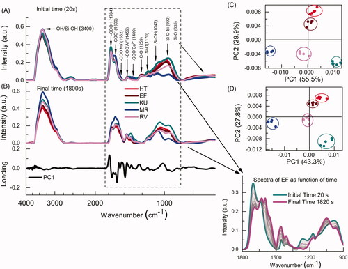
Figure 2. (A) Curve representing the time evolution for the values of PC1 in the PCA analysis calculated from the FTIR-ATR. Each curve is an average of five independent measurements (n = 5). The exponential fitting with EquationEquation (1)(1) provided the stabilization time of chemical bonds (τ) of the GICS; (B) Comparison between the hardening times and the stabilization times.
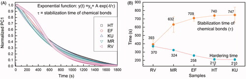
Figure 3. GICs temperature variation as a function of time. The inserts exemplify images obtained by the thermographic camera at specific instants of the reaction.
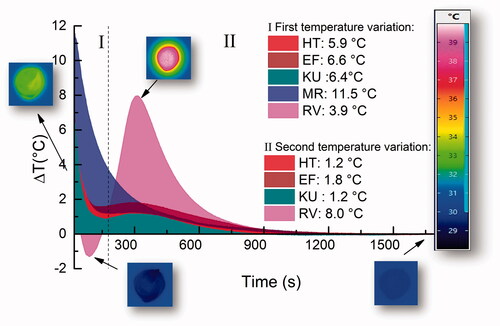
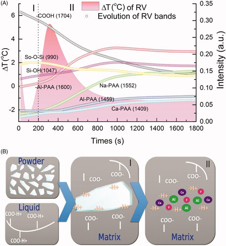
Figure 4. (A) Comparison between the temperature variation of RV and the evolution of the bands as a function of time; (B) schematic illustration of possible sequences of the reaction. (I) First stage of the reaction, which is the acid hydrolysis on the glass particles surfaces; (II) second stage representing the ion release to the matrix.