What Quantity Appears on the Vertical Axis of a Normal Distribution? A Student Survey

Figures & data

Fig. 1 Answers to survey Question 1: label vertical axis.

NOTE: This bar chart shows counts (and proportions) of students giving vertical axis labels in response to survey Question 1. Of the 148 students surveyed, “Frequency” and “Count,” if combined, were the most popular incorrect responses. The single most popular incorrect answer was, however, “Probability.” The “Other” category include nonsensical answers like “Ethnicity” or “Weight” or “Kurtosis,” and also two students who left the answer blank. See also Table 2 for a breakdown of answers to Question 1 by degree program.

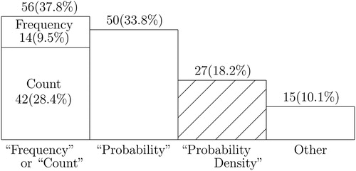
Fig. 2 Number of correct survey answers per student.

NOTE: This probability mass function shows the proportion of our sample of 148 students getting 0, 1, 2, 3, or 4 correct answers, respectively, to the four questions posed in our probability density survey. Counts are shown in parentheses. The mean of 0.38 correct answers per student is indicated with a small triangle. The median number of correct answers per student was 0.

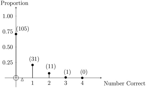
Table 3 Which survey answers students got correct.

No. Correct	Q1	Q2	Q3	Q4	Count
0	N	N	N	N	105
1	Y	N	N	N	15
1	N	Y	N	N	2
1	N	N	N	Y	14
2	Y	Y	N	N	4
2	Y	N	Y	N	1
2	Y	N	N	Y	6
3	Y	Y	Y	N	1
4	Y	Y	Y	Y	0

NOTE: This table summarizes actual outcomes to the four survey questions. “Y” means yes, the answer was correct; “N” means no, the answer was incorrect. As summarized in Figure 2, 105 students got no correct answers, $15+2+14=31$ students got one correct answer, $4+1+6=11$ students got two correct answers, 1 student got three answers correct, and no students got four correct answers. Although there are 16 possible permutations of Y and N over the four questions, we saw only the eight outcomes shown here. As mentioned earlier, only $4+1=5$ students could both label the vertical axis (Q1) and explain their answer (Q2), and only $15+4+1+6+1=27$ students could answer Q1 correctly.

Table 1 Proportion of students answering correctly.

Question	Statistics	Physics	Finance	MF	Overall
Q1	6 (42.9%)	4 (25.0%)	12 (12.0%)	5 (27.8%)	27 (18.2%)
Q2	0 (0.0%)	1 (6.3%)	5 (5.0%)	1 (5.6%)	7 (4.7%)
Q3	0 (0.0%)	2 (12.5%)	0 (0.0%)	0 (0.0%)	2 (1.4%)
Q4	0 (0.0%)	1 (6.3%)	18 (18.0%)	1 (5.6%)	20 (13.5%)
Overall	10.7%	12.5%	8.8%	9.7%	9.5%
N	14 (9.5%)	16 (10.8%)	100 (67.6%)	18 (12.2%)	148 (100.0%)

NOTES: This table shows the count and proportion of students giving the correct answers to the four survey questions, by degree program: statistics, physics, and finance undergraduates, and master of finance (MF). For example, with four questions asked of each student, it follows that $(4+1+2+1)/(16\times 4)=12.5\%$ of all questions asked of physics majors were answered correctly, as reported overall. N is the count of students in each program, with proportions in parentheses. See Appendix A.2 to link question numbers to question content. See also Table 2 for a further breakdown of answers to Question 1.

Table 2 Breakdown of answers to Question 1 by degree program.

Answer	Statistics	Physics	Finance	MF	Overall
“Probability density”	6 (42.9%)	4 (25.0%)	12 (12.0%)	5 (27.8%)	27 (18.2%)
“Probability”	1 (7.1%)	8 (50.0%)	34 (34.0%)	7 (38.9%)	50 (33.8%)
“Count”	4 (28.6%)	2 (12.5%)	34 (34.0%)	2 (11.1%)	42 (28.4%)
“Frequency”	3 (21.4%)	1 (6.3%)	6 (6.0%)	4 (22.2%)	14 (9.5%)
Other	0 (0.0%)	1 (6.3%)	14 (14.0%)	0 (0.0%)	15 (10.1%)
N	14 (9.5%)	16 (10.8%)	100 (67.6%)	18 (12.2%)	148 (100.0%)

NOTES: This table shows the count and proportion of student responses to Question 1 of our survey (i.e., label the vertical axis of a normal distribution). The correct answer is “probability density,” and the most common incorrect answers were “probability,” “count,” and “frequency.” Some of the other nonsense answers were mentioned already in the caption to Figure 1. The data are broken down by degree program: statistics, physics, and finance undergraduates, and master of finance (MF). N is the count of students in each program, with proportions in parentheses.

Fig. 3 Probability mass function $P(X_d=x).$

NOTE: The discrete random variable X_d takes values $x=1,2,$ and 4, with probabilities $\frac{1}{4},\frac{1}{4}$, and $\frac{1}{2}$, respectively. The triangle marks the probability-weighted average of the distribution (i.e., the mean of 2.75); this is the location of the perpendicular axis through the center of gravity of the probability mass distribution. The corresponding cumulative distribution function appears in Figure 4.

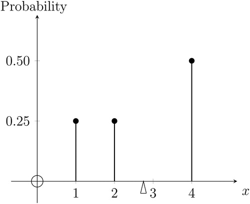
Fig. 4 Cumulative distribution function $P(X_d\le x).$

NOTE: The discrete random variable X_d takes values $x=1,2,$ and 4, with probabilities $\frac{1}{4},\frac{1}{4}$, and $\frac{1}{2}$, respectively. The plot shows the cumulative distribution function $P(X_d\le x)$. The corresponding pmf appears in Figure 3.

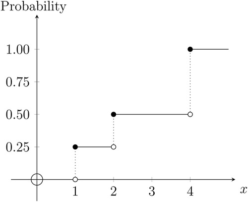
Fig. 5 Normal cumulative distribution function $F_X(x).$

NOTE: The cdf $F_X(x)$ is illustrated for a normal distribution with mean μ and standard deviation σ (see Equation (1)(1) $$\begin{array}{c}{F}_X(x)=P(X\le x)={\int }_{t=-\infty }^x\frac{1}{\sqrt{2\pi }\sigma }{e}^{-\frac{1}{2}{\left(\frac{t-\mu }{\sigma }\right)}^2}dt,\\ -\infty <x<\infty \end{array}$$(1) ). The slope of the cdf is close to zero at points a and c and reaches a maximum of $1/\left(\sqrt{2\pi }\sigma \right)$ at point b.

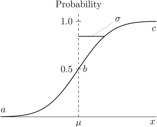
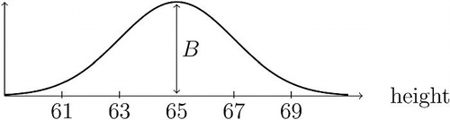
Fig. 6 Normal pdf $f_X(x).$

NOTE: A pdf $f_X(x)$ is illustrated for normally distributed X with mean μ and standard deviation σ (see Equation (2)(2) $$f_X(x)=\frac{1}{\sqrt{2\pi }\sigma }{e}^{-\frac{1}{2}{\left(\frac{x-\mu }{\sigma }\right)}^2},-\infty <x<\infty$$(2) ). The height of the pdf is close to zero at points a and c, and reaches a maximum of $1/\left(\sqrt{2\pi }\sigma \right)$ at point b.

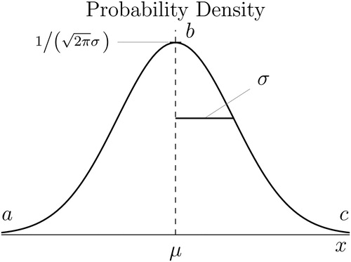
Fig. 7 Zoomed View of the ith narrow slice under $f_X(x).$

NOTE: We assume a discretization of the x-axis under $f_X(x)$ into small steps numbered using i, where x_i sits at the center of the ith small step. $f_X(x_i)$ is the height of the function f_X at x_i, $\Delta x_i$ is the width of the ith small step centered on x_i, and ${\text{area}}_i$ is the area of the ith narrow slice centered on x_i. We assume $P(x_i;\Delta x)\equiv P\left(x_i-\frac{\Delta x}{2}\le X\le x_i+\frac{\Delta x}{2}\right)$, as in Equation (3)(3) $$P(x_i;\Delta x)\equiv P\left(x_i-\frac{\Delta x}{2}\le X\le x_i+\frac{\Delta x}{2}\right),$$(3) .

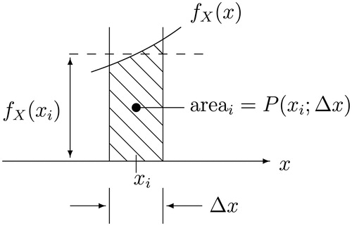
Fig. 8 Rescaling preserves Shape I.

NOTE: The left-hand-side density plot shows height of female undergraduates measured in inches; the right-hand-side density plot shows their height measured in centimeters (see the text). The two figures have an identical shape; all that changes are the scales on the axes. Challenge: Can you confirm that if height is instead measured in meters, we expect the peak height of the second pdf to be roughly $8{\text{meters}}^{-1}$?

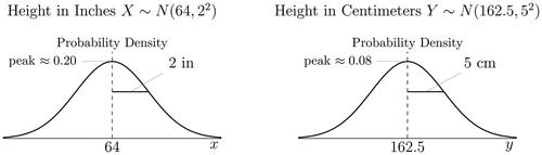
Fig. 9 Rescaling preserves Shape II.

NOTE: The left-hand-side density plot shows the uniform density U(0, 2) with pdf $f_X(x)=\frac{1}{2}$ for $0\le x\le 2$ and 0 otherwise. The right-hand-side density plot shows the uniform density U(0, 4) with pdf $f_Y(y)=\frac{1}{4}$ for $0\le y\le 4$ and 0 otherwise. X counts half-revolutions of a dart’s impact point around a dartboard and Y counts quarter-revolutions (see the text).

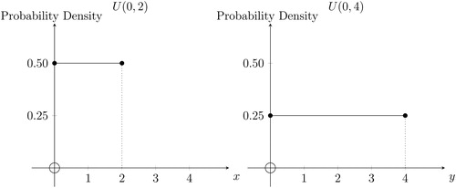
Fig. A1 Height of female students, measured in centimeters.

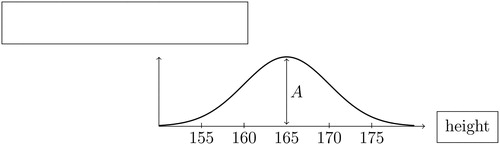
Fig. A2 Height of female students, measured in inches.