Diamond quantum sensors: from physics to applications on condensed matter research

Figures & data

Figure 1. (a) The structure of the NV centre in the diamond crystal, which contains a substitution N atom directly connected to a vacancy with $C_{3v}$ symmetry. (b) The simplified level structure of the NV centre. Its unique transitions lead to optical spin initialisation and readout. The optically detected magnetic resonance (ODMR) measurement is enabled by scanning MW of frequencies across the resonant frequencies between $|0〉$ and $|\pm 1〉$ ground states.

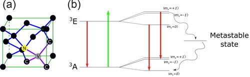
Figure 2. An illustration of the versatility of the NV centre, including magnetic field sensing under pressure (Reproduced with permission from Yip et al., Science 366, 1355 (2019). Copyright 2019 American Association for the Advancement of Science), electric field sensing (Reproduced with permission from Dolde et al., Nat. Phys. 7, 459 (2011). Copyright 2011 Springer Nature, stress sensing (Reproduced from Barson et al., Nano Lett. 17, 1496 (2017). Copyright 2017 Author(s), licensed under a Creative Commons Attribution (CC BY) license), temperature sensing (Reproduced from Neumann et al., Nano Lett. 13, 2738 (2013). Copyright 2013 Author(s), licensed under a Creative Commons Attribution (CC BY) license) and magnetic imaging (Reproduced from Wang et al., Sci. Adv. 5, eaau8038 (2019). Copyright 2019 Author(s), licensed under a Creative Commons Attribution (CC BY) license).

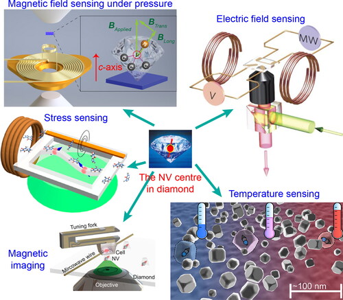
Figure 3. Hahn echo, whose basic sequence is ${\frac{\pi }{2}}_x-\frac{\tau }{2}-{\pi }_x-\frac{\tau }{2}-{\frac{\pi }{2}}_x$ where π represents a microwave pulse of sufficient duration to rotate the state along x-axis for π on Bloch Sphere and τ is free evolution time.

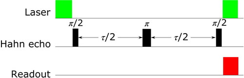
Figure 4. The Carr-Purcell-Meiboom-Gill (CPMG) pulse sequence. The sequence of CPMG is ${\frac{\pi }{2}}_x-{(\frac{\tau }{2n}-{\pi }_y-\frac{\tau }{2n})}^n-{\frac{\pi }{2}}_x$ and the interval duration between each two π pulse is equal. The CPMG pulse sequence is proved to extend the coherence time longer by eliminating high order fluctuating noise.

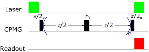
Figure 5. Knill dynamical decoupling (KDD) sequence. This KDD method is robust against pulse errors and is symmetric for arbitrary initial superposition states.

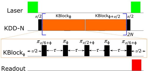
Figure 6. (a) Left: Schematic drawing of the setup. A YIG thin film was placed below a diamond chip, containing NV centres at 20 nm below the surface. NV centres detected the magnetic stray field from the spin waves results from PL drops at certain frequencies. Right: A gold stripline was used to generate spin waves. An external magnetic field was aligned with one of the four possible NV orientations. (b) Spin-wave frequency verse wave number. The red line was the calculated spin-wave dispersion. (c) Normalized NV PL using pulsed control verse distance from the stripline and delay time, showing the spin-wave dispersion in both space and time domains. Reproduced from Bertelli et al., Sci. Adv. 6, eabd3556 (2020). Copyright 2020 Author(s), licensed under a Creative Commons Attribution (CC BY) license. (d) Left: Schematic drawing of using the NV sensor to locally probe the magnons of a YIG thin film. Right: Normalized NV PL as a function of external magnetic field and microwave frequency. The calculated dispersion agreed with the observed features. Reproduced from Lee-Wong et al., Nano Lett. 20, 3284 (2020). Copyright 2020 Author(s), licensed under a Creative Commons Attribution (CC BY) license.

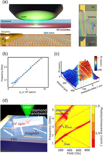
Figure 7. (a) An 661-nm excitation laser was used to generate a temperature distribution within Mos₂, driving a circulating photocurrent distribution. The NV centre probed the magnetic field produced by the photocurrent and optically read out by a ­532-nm probe laser. (b) Room-temperature PL of the boundary between Mos₂ and an ensemble NV centre under 532-nm illumination. This graph justified the use of 661-nm excitation wavelength (longer than NV ZPL at 637 nm) to minimize optical excitation. The orange shaded region represented the NV PL collection region. (c) Comparison of the current density model $\overrightarrow{J}$ which best fits the data, the simulated laser-induced temperature distribution T_M, and the power density PD of the excitation laser. The current density model was in close agreement with the temperature gradient, also agreed with the experiential data. Reproduced from Zhou et al., Phys. Rev. X 10, 011003 (2020). Copyright 2020 Author(s), licensed under a Creative Commons Attribution (CC BY) license.

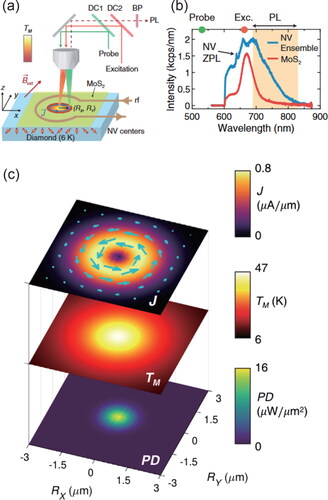
Figure 8. (a) Schematic drawing of the experimental setup. The NDs were spread throughout the surface. The deformation caused by the localized indentation of an AFM tip was sensed by the rotation of NDs. (b) AFM image of a polydimethylsiloxane (PDMS) surface with an ND located at the centre, showing the sequence of the indentation from # 1 to # 92. (c) The rotation of the ND. The arrow represented both the magnitude of the rotation angle and the direction. (d) The reconstructed surface of the PDMS film upon AFM tip indentation at the centre. Reproduced from Xia et al., Nat. Commun 10, 3259 (2019). Copyright 2019 Author(s), licensed under a Creative Commons Attribution (CC BY) license. (e) The NDs were placed in a homemade perfusion chamber that simultaneously allows the exchange of the solution and the optical experiment. (f) ODMR spectra of the ND when it is fixed on the coverslip (top) and is about to detach (bottom). The reduction of contrast and broaden of linewidth can be observed clearly. Reproduced from Fujiwara et al., Sci. Rep. 8, 14773 (2018). Copyright 2018 Author(s), licensed under a Creative Commons Attribution (CC BY) license.

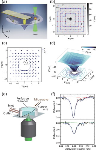
Figure 9. (a) ZFC-W and FC-C measurements in LuNi₂B₂C probed at the sample centre. The splitting verse temperature showed the Meissner effect, where T_c is found to be 16.6 ± 0.1 K. The inset was the ODMR spectrum. (b) The spatial FC profile at 100 Oe. The sample was located at $x\ge 0$ and the Meissner expulsion was visible near the edge. The inset was the Zeeman splitting with decreasing temperature. Reproduced from Nusran et al., New J. Phys. 20, 043010 (2018). Copyright 2018 Author(s), licensed under a Creative Commons Attribution (CC BY) license. (c) ZFC measurements of $H_{c1}$ of Ba(Fe${}_{1-x}$Co_x)₂As₂ at 4.5 K. A, B, C, and D represented four different points near the edge and all the Zeeman splitting agreed well. The inset was the averaged signal of Z_S. The $H_p=13.2\pm 1$ Oe was determined from the sudden change. Reproduced with permission from Joshi et al., Phys. Rev. Appl. 11, 014035 (2019). Copyright 2019 American Physical Society. (d) Left: Calculated magnetic field distribution on top of a superconducting circular disk at 40 K (red curve) and 70 K (blue curve). Left: PL image of the BSSCO film at 40 and 70 K. Reproduced from Xu et al., Nano Lett. 19, 5697 (2019). Copyright 2019 Author(s), licensed under a Creative Commons Attribution (CC BY) license.

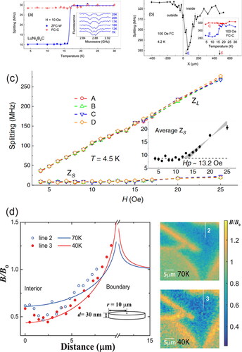
Figure 10. (a) Image of the magnetic stray field from a single vortex obtained with the NV magnetometer. (b) 3 D reconstruction of the vortex obtained as in (a). (c) Vertical scan through the vortex stray field in the $x-z$ plane indicated in (b). Reproduced with permission from Thiel et al., Nat. Nanotechnol 11, 677 (2016). Copyright 2016 Springer Nature. (d) Three images of vortices that were taken for different magnetic fields presented during the cooling process. An increase in the number of vortices can be observed when the field is increased. The observed number of vortices agreed excellently with the expected number of vortices. Reproduced with permission from Schlussel et al., Phys. Rev. Appl. 10, 034032 (2018). Copyright 2018 American Physical Society.

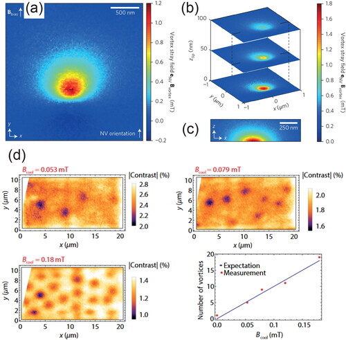
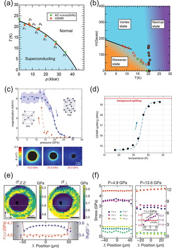
Figure 11. (a) The T – P phase diagram of the BaFe₂(As${}_{0.59}$P${}_{0.41}$)₂ sample measured by ac susceptibility and ODMR methods, showing good agreement between common method and the novel ODMR method. (b) The H – P phase diagram of the same sample measured by the ODMR method. This work opened up a discussion of the superconducting gap function. Reproduced withpermission from Yip et al., Science 366, 1355 (2019). Copyright 2019 American Association for the Advancement of Science. (c) The magnetization versus pressure of an iron bead sample. The expected hysteresis of the structural transition can be observed from the difference between increasing and decreasing pressure. (d) The evolution of the ODMR splitting versus temperature of a MgB₂ sample. Reproduced with permission from Lesik et al., Science 366, 1359 (2019). Copyright 2019 American Association for the Advancement of Science. (e) Spatially resolved maps of the loading stress (left) and mean lateral stress (right), across the culet surface. A linecut along the white-dashed line of the two stresses is highlighted (bottom). These results agreed with the finite-element analysis. (f) Comparison of the full stress tensor along the dotted line at two different pressures. A noticeable pressure gradient was observed at higher pressure, meaning the pressure medium had entered the glassy phase. Reproduced with permission from Hsieh et al., Science 366, 1349 (2019). Copyright 2019 American Association for the Advancement of Science.