Role of Variable Renewable Energy Penetration on Electricity Price and its Volatility across Independent System Operators in the United States

Figures & data

Table 1. Temporal range, resolution, and VRE composition for ISO data.

ISO	Date range	Original resolution	VRE	Reference
New England Independent System Operator, ISONE	2014–2020	hourly	Solar and wind	ISONE (2021)
New York Independent System Operator, NYISO	2015–2020	5 mins	Wind	NYISO (2020)
Pennsylvania, Jersey, Maryland Power Pool, PJM	2016–2018	hourly	solar and wind	PJM (2021)
Midcontinent Independent System Operator, MISO	2015–2019	hourly	Wind	MISO (2021)
Southwest Power Pool, SPP	2019–2020	5 mins	Solar and wind	SPP (2021)
California Independent System Operator, CAISO	2017–2020	5 mins	Solar and wind	California ISO (2017)

Table 2. Literature summary for US studies (domestic) on VRE impact on price. The specified VRE, solar or wind, is given in the rightmost column.

Author	Region	Time period	Decrease in system electricity price per GWh of specified VRE
Zarnikau et al. (2020)	MISO	2013–2017	Wind (DAM): $2.1–$6
Bushnell and Novan (2018)	CAISO	2012–2016	Solar: $0.1
Haratyk (2017)	Midwest, Mid Atlantic	2008–2015	Wind (Midwest): $0.612, Wind (Mid-Atlantic): $ 0
Quint and Dahlke (2019)	MISO	2008–2016	Wind: $1.4–$3.4
Tsai and Eryilmaz (2018)	ERCOT	2014–2016	Wind: $1.45–$4.45
Zarnikau et al. (2019)	ERCOT	2011–2017	Wind: $1.64
Woo et al. (2011)	ERCOT	2007–2010	Wind (Houston): $3.9
			Wind (north):$ 6.1
			Wind (south): $3.2
			Wind (west): $15.3
Woo et al. (2013)	Mid-C Hub	2006–2012	Wind (day): $0.96
			Wind (night): $0.72
Woo et al. (2014)	CAISO	2010–2012	Solar (NP15): $12.4
			Wind (NP15): $7.8
			Solar (SP15): $12.2
			Wind (SP15): $9.8
			Solar (ZP26): $14.3
			Wind (ZP26): $7.9
Woo et al. (2016)	CAISO	2012–2015	RTM Solar (NP15): $2.2
			Wind (NP15): $2.8 Solar (SP15): $3.7 Wind (SP15): $1.5 DAM Solar (NP15): $5.3 Wind (NP15): $3.3 Solar (SP15): $3.2 Wind (SP15): $1.4

Note: RTM = real time market; DAM = day ahead market.

Figure 1. Map of independent system operators (ISOs) in the United States. ISOs are responsible for coordinating, controlling, and monitoring the electricity grid within their region of control. There are seven ISOs in the United States, and the regions covered by these ISOs account for 67% of the total electricity demand in the country. Adapted from Climate-XChange (2021).

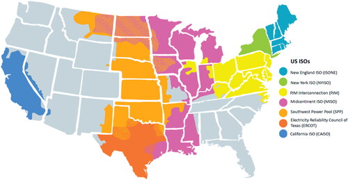
Figure 2. The energy price data for each ISO is detrended by the average price for hour, season, and weekend trends. The observed price data, shown with black dots, is plotted by day of the year. The red line indicates the estimated trend. The resulting detrended price is the observed value minus the average. Note there are repeated observations for multiple years and the y-axis is clipped to the range $10–150.

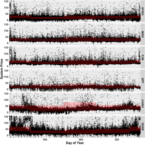
Figure 3. CAISO raw system prices by seasons and hour of day. The plot shows the estimated diurnal pattern (red line) by season. For plotting purposes, prices greater than 150 are excluded. Orange dots depict negative prices and teal dots depict positive prices (all in USD).

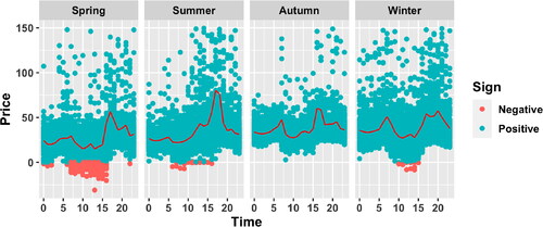
Figure 4. Quantiles of skew t-distribution based on the estimated pointwise means of the parameters listed in Table A1. Points correspond to seasonally detrended system price and the y-axis is trimmed to the inner 99% of detrended price; red points correspond to a negative price before seasonal detrending.

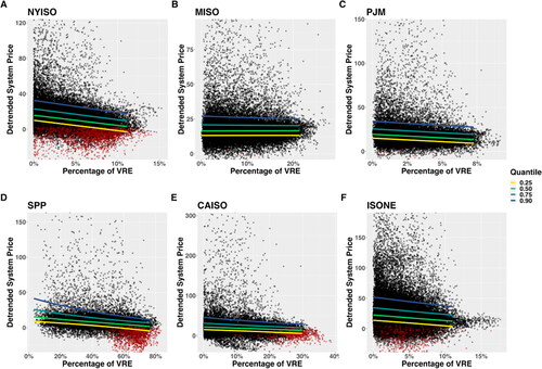
Figure 5. VRE (solar and wind) penetration. Shown here is the percentage of VRE generation to total generation in each of the six ISOs considered. Southwest Power Pool (SPP) achieved the highest VRE penetration based on the data used and for the study period considered, followed by CAISO, MISO, ISONE, NYISO, and PJM.

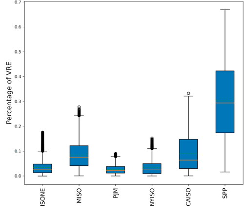
Table 3. Descriptive Statistics Summary. This shows the minimum, median, maximum, and mean statistics for the detrended system price (in USD) and temporal price volatility (in USD).

		CAISO	ISONE	MISO	NYISO	PJM	SPP
	min	−76.29	−208.37	−33.51	−2504.87	−78.80	−49.36
	median	−5.14	−4.82	−1.74	−1.02	−2.79	−2.63
	max	957.62	2,396.98	546.73	1,145.75	615.95	1,086.95
	mean	0.00	0.00	0.00	0.00	0.00	0.00
Detrended price ($)	st. dev.	41.34	34.26	14.73	36.26	20.28	27.27
	min	0.19	0.15	0.13	0.18	0.11	0.23
	median	1.83	1.67	1.17	1.59	1.36	1.72
	max	24.92	33.79	18.69	37.21	19.30	27.50
	mean	2.36	1.95	1.49	1.93	1.72	2.17
Price volatility ($)	st. dev.	2.13	1.29	1.18	1.52	1.26	1.73
	min	0.04	0.00	0.04	0.00	0.01	3.10
	median	7.28	2.74	7.56	2.44	2.22	48.15
	max	38.51	17.64	27.78	15.24	9.16	83.30
	mean	10.04	3.37	8.47	3.27	2.62	46.38
Percentage of VRE (%)	st. dev.	8.10	2.58	5.24	2.82	1.79	16.81

Figure 6. VRE penetration (in %) and detrended electricity price (in $). The six panels show the relationship between VRE penetration and detrended electricity price for NYISO, MISO, PJM, CAISO, ISONE, and SPP, respectively. The continuous lines show the quantiles with the colors yellow, green, blue, and purple, representing the 0.25th, 0.50th (median), 0.75th, and the 0.90th quantiles, respectively. Each panel’s axis limits are adjusted separately in order to clearly show the quantiles’ trend direction.

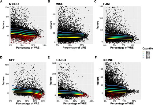
Figure 7. The derivative of the detrended system price (in USD) and detrended system price volatility (temporal volatility in USD) with respect to the percentage of VRE for the PJM independent system operator.

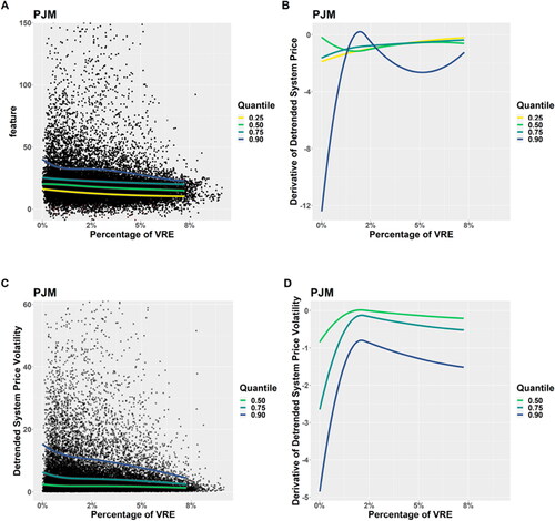
Figure 8. Estimated effects of VRE percentage on the skewness (ν) parameter for a skew t-distribution for detrended price using a log link. Gray bands indicate the 95% confidence intervals. The red reference line at 1 denotes symmetry.

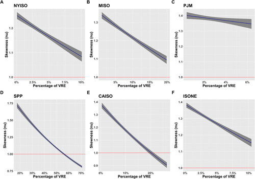
Figure 9. VRE penetration (in %) and temporal price volatility (in USD). The panels show the relationship between VRE penetration and temporal detrended system price volatility for NYISO, MISO, PJM, CAISO, ISONE, and SPP, respectively. The continuous lines show the quantiles with the colors yellow, green, and purple, representing the 0.50th (median), 0.75th and the 0.90th quantiles.

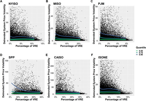
Figure 10. Difference between 0.75th and 0.25th quantile (yellow), 0.75th and 0.50th (teal), and 0.90th and 0.50th (purple) as plotted with approximate 95% credible intervals. It is important to note that for several of the ISOs, a decrease in the spread of the distribution (volatility with respect to VRE) is observed in the quantiles as measured by all three differences, but SPP and CAISO have curvilinear trends in the difference between 0.75th and 0.25th, which is caused by the skewness changing from positive to negative with increasing VRE penetration.

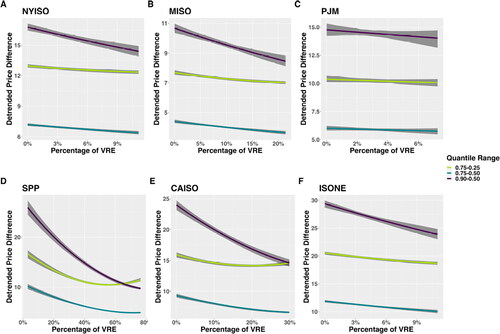
Figure A1. The three panels show an illustration of the detrending procedure for a snapshot of data from CAISO in the second half of July 2019. In (A) the raw system price is shown (dots) along with the estimated seasonal trend (red line). We detrend the raw system price by subtracting the trend to obtain the detrended system price (B). The detrended system price represents how much the system price differs from the seasonal average; note that most of the time it is near 0. From (B), we calculated the exponentially weighted moving average standard deviation (C) that is a temporal measure of the variability of the detrended system price- in other words, How much does the detrended price vary from the detrended prices in the recent past?

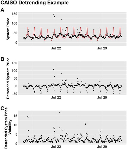
Table A1. Parameter values for the generalized skew t-distribution hourly detrended price. An example of interpretation of the effect of VRE on the centrality and skewness of the distribution of hourly price is an increase in VRE decreases both centrality and skewness of hourly price in CAISO (${\beta }_1^{\mu }<0$ and ${\beta }_1^{\nu }<0$). The interpretation also holds for ISONE, NYISO and SPP.

	Parameter	Estimate	Std. Error
ISO	${\beta }_0^{\mu },$ centrality intercept	–5.74	0.18
	${\beta }_1^{\mu },$ change in centrality for a change in VRE	–5.14	1.59
	${\beta }_0^{\sigma },$ log-scale estimate	2.10	0.01
	${\beta }_0^{\nu },$ skewness intercept	0.25	0.01
	${\beta }_1^{\nu },$ change in skewness for a change in VRE	–1.58	0.11
CAISO	${\beta }_0^{\tau },$ log-tail index estimate	0.52	0.01
	${\beta }_0^{\mu },$ centrality intercept	–7.48	0.18
	${\beta }_1^{\mu },$ change in centrality for a change in VRE	–62.56	4.17
	${\beta }_0^{\sigma },$ log-scale estimate	2.42	0.01
	${\beta }_0^{\nu },$ skewness intercept	0.33	0.01
	${\beta }_1^{\nu },$ change in skewness for a change in VRE	–1.75	0.22
ISONE	${\beta }_0^{\tau },$ log-tail index estimate	0.72	0.01
	${\beta }_0^{\mu },$ centrality intercept	–4.04	0.12
	${\beta }_1^{\mu },$ change in centrality for a change in VRE	7.57	1.10
	${\beta }_0^{\sigma }$, log-scale estimate	1.47	0.01
	${\beta }_0^{\nu },$ skewness intercept	0.30	0.02
	${\beta }_1^{\nu },$ change in skewness for a change in VRE	–1.07	0.14
MISO	${\beta }_0^{\tau },$ log-tail index estimate	0.78	0.01
	${\beta }_0^{\mu },$ centrality intercept	–0.38	0.14
	${\beta }_1^{\mu }$, change in centrality for a change in VRE	–98.38	3.58
	${\beta }_0^{\sigma },$ log-scale estimate	2.05	0.01
	${\beta }_0^{\nu },$ skewness intercept	0.23	0.01
	${\beta }_1^{\nu },$ change in skewness for a change in VRE	–1.44	0.26
NYISO	${\beta }_0^{\tau },$ log-tail index estimate	0.89	0.01
	${\beta }_0^{\mu },$ centrality intercept	–4.15	0.17
	${\beta }_1^{\mu },$ change in centrality for a change in VRE	–79.23	5.13
	${\beta }_0^{\sigma },$ log-scale estimate	1.74	0.01
	${\beta }_0^{\nu },$ skewness intercept	0.33	0.02
	${\beta }_1^{\nu },$ change in skewness for a change in VRE	–0.49	0.51
PJM	${\beta }_0^{\tau },$ log-tail index estimate	0.75	0.02
	${\beta }_0^{\mu },$ centrality intercept	–2.88	0.28
	${\beta }_1^{\mu },$ change in centrality for a change in VRE	–5.18	0.87
	${\beta }_0^{\sigma },$ log-scale estimate	1.86	0.01
	${\beta }_0^{\nu },$ skewness intercept	0.64	0.03
	${\beta }_1^{\nu },$ change in skewness for a change in VRE	–1.63	0.08
SPP	${\beta }_0^{\tau },$ log-tail index estimate	0.77	0.02

ISONE. 2021. ISO New England Web Services API v1.1. https://webservices.iso-ne.com/docs/v1.1/.

 Google Scholar

NYISO. 2020. OASIS (Open Access Same-Time Information System). http://mis.nyiso.com/public/.

 Google Scholar

PJM. 2021. Data Miner 2. https://dataminer2.pjm.com/list.

 Google Scholar

MISO. 2021. Markets and operations. https://www.misoenergy.org/markets-and-operations/#t=10&p=0&s=&sd=.

 Google Scholar

SPP. 2021. SPP integrated marketplace. https://marketplace.spp.org/.

 Google Scholar

California ISO. 2017. Interface Specification for OASIS Fall Spring 2017 Release, Technical report. http://www.caiso.com/Documents/InterfaceSpecifications-OASISv3_12_0.pdf.

 Google Scholar

Zarnikau J, Tsai C, Woo C. 2020. Determinants of the wholesale prices of energy and ancillary services in the U.S. Midcontinent electricity market. Energy. 195:117051. https://www.sciencedirect.com/science/article/pii/S0360544220301584?via%3Dihub#bib19.

 Web of Science ®Google Scholar

Bushnell J, Novan K. 2018. Setting with the sun: the impacts of renewable energy on wholesale power markets, Technical report. National Bureau of Economic Research.

 Google Scholar

Haratyk G. 2017. Early nuclear retirements in deregulated U.S. markets: causes, implications and policy options. Energy Policy. 110:150–166. https://www.sciencedirect.com/science/article/pii/S0301421517305177?via%3Dihub.

 Web of Science ®Google Scholar

Quint D, Dahlke S. 2019. The impact of wind generation on wholesale electricity market prices in the midcontinent independent system operator energy market: an empirical investigation. Energy. 169:456–466. https://www.sciencedirect.com/science/article/pii/S0360544218323946.

 Web of Science ®Google Scholar

Tsai C-H, Eryilmaz D. 2018. Effect of wind generation on ERCOT nodal prices. Energy Econ. 76:21–33. https://www.sciencedirect.com/science/article/pii/S0140988318303931?via%3Dihub.

 Web of Science ®Google Scholar

Zarnikau J, Woo C, Zhu S, Tsai C. 2019. Market price behavior of wholesale electricity products: Texas. Energy Policy. 125:418–428. https://www.sciencedirect.com/science/article/pii/S0301421518306980?via%3Dihub.

 Web of Science ®Google Scholar

Woo C, Horowitz I, Moore J, Pacheco A. 2011. The impact of wind generation on the electricity spot-market price level and variance: the Texas experience. Energy Policy. 39(7):3939–3944. https://www.sciencedirect.com/science/article/pii/S0301421511002813?via%3Dihub.

 Web of Science ®Google Scholar

Woo C-K, Zarnikau J, Kadish J, Horowitz I, Wang J, Olson A. 2013. The impact of wind generation on wholesale electricity prices in the Hydro-Rich Pacific Northwest. IEEE Trans Power Syst. 28(4):4245–4253. https://ieeexplore.ieee.org/document/6529186/.

 Web of Science ®Google Scholar

Woo C, Ho T, Zarnikau J, Olson A, Jones R, Chait M, Horowitz I, Wang J. 2014. Electricity-market price and nuclear power plant shutdown: evidence from California. Energy Policy. 73:234–244. https://www.sciencedirect.com/science/article/pii/S0301421514003085?via%3Dihub.

 Web of Science ®Google Scholar

Woo C, Moore J, Schneiderman B, Ho T, Olson A, Alagappan L, Chawla K, Toyama N, Zarnikau J. 2016. Merit-order effects of renewable energy and price divergence in California’s day-ahead and real-time electricity markets. Energy Policy. 92:299–312. https://www.sciencedirect.com/science/article/pii/S0301421516300635?via%3Dihub.

 Web of Science ®Google Scholar

Climate-Xchange. 2021. ISO Maps. https://climate-xchange.org/independent-system-operators-isos-carbon-pricing-an-explainer/iso-maps-v4_isos/.

 Google Scholar

Data availability statement

Raw data and code can be found here: https://github.com/Qunlexie/VRE-Impact-on-Price-and-Volatility.