A clustering algorithm for overlapping Gaussian mixtures

Figures & data

Fig. 1 (a) The contour plots of the three subpopulations given the label of the observations generated under the distribution scheme of Example 1. (b) The clusters obtained by the K-means. (c) The clusters obtained by the GMM. (d) The clusters obtained by the proposed algorithm.

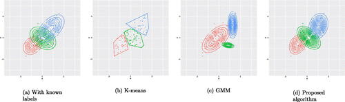
Fig. 2 (a) The contour plots of the three subpopulations given the label of the observations generated under the distribution scheme of Example 2. (b) The clusters obtained by the K-means. (c) The clusters obtained by the GMM. (d) The clusters obtained by the proposed algorithm.

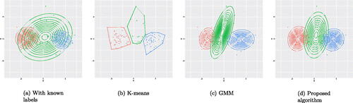
Fig. 3 (a) The contour plots of the three subpopulations given the label of the observations generated under the distribution scheme of Example 3. (b) The clusters obtained by the K-means. (c) The clusters obtained by the GMM. (d) The clusters obtained by the proposed algorithm.

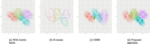
Fig. 4 (a) The scatterplot of the three subpopulations given the label of the observations generated under the distribution scheme of Example 1. (b) A rejected data partition. (c) A not-rejected data partition. (d) The kernel density plot for the observed data. (e) The kernel density plot for the rejected artificial data set generated using the partition presented in subfigure (b). (f) The kernel density plot for the not-rejected artificial data set generated using the partition presented in subfigure (c).

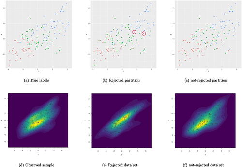
Table 1 Summary results (Mean values-upper tabular, standard deviations-second tabular, and performance evaluation metrics-two bottom tabular) for the 1000 simulated samples from Scenario 1.

Mean values
	1st cluster						2nd cluster						3rd cluster
	n	μx	μy	σ11	σ12	σ22	n	μx	μy	σ11	σ12	σ22	n	μx	μy	σ11	σ12	σ22
True	40	−4	0	1	0	1	40	0	0	4	0	4	40	4	0	1	0	1
K-means	42.38	–3.93	–0.00	0.99	–0.00	1.05	35.06	–0.01	0.01	1.04	0.01	1.86	42.56	3.93	–0.00	1.00	0.00	1.05
GMM	44.47	–3.81	0.00	1.11	0.01	1.01	31.18	0.01	0.01	0.73	0.01	1.93	44.35	3.82	0.00	1.11	–0.01	1.00
New	42.38	–3.94	–0.00	0.97	0.01	1.04	35.47	0.02	0.00	1.07	0.01	1.91	42.14	3.96	0.00	0.97	–0.01	1.03
St. Dev. of the estimates
	n	μx	μy	σ11	σ12	σ22	n	μx	μy	σ11	σ12	σ22	n	μx	μy	σ11	σ12	σ22
K-means	3.53	0.21	0.21	0.28	0.17	0.24	3.16	0.49	0.31	0.25	0.23	0.48	3.75	0.24	0.18	0.30	0.18	0.25
GMM	5.72	0.34	0.18	0.55	0.22	0.25	8.25	0.53	0.37	0.41	0.39	0.66	5.99	0.34	0.17	0.53	0.22	0.25
New	2.38	0.19	0.17	0.19	0.16	0.24	2.93	0.29	0.28	0.19	0.24	0.47	2.41	0.19	0.16	0.19	0.17	0.24

Table

Performance evaluation metrics
	Sensitivity	Specificity	Recall	F1	Sensitivity	Specificity	Recall	F1	Sensitivity	Specificity	Recall	F1
K-means	0.97	0.82	0.97	0.96	0.97	0.95	0.97	0.82	0.97	0.94	0.87	0.94
GMM	0.98	0.73	0.98	0.93	0.98	0.93	0.98	0.73	0.98	0.93	0.81	0.93
New	0.98	0.84	0.97	0.96	0.97	0.96	0.98	0.84	0.97	0.95	0.89	0.95

Table 2 Summary results (Mean values-upper tabular, standard deviations-second tabular, and performance evaluation metrics-two bottom tabular) for the 1000 simulated samples from Scenario 2.

Mean values
	1st cluster						2nd cluster						3rd cluster
	n	μx	μy	σ11	σ12	σ22	n	μx	μy	σ11	σ12	σ22	n	μx	μy	σ11	σ12	σ22
True	40	–4	0	1	0	1	40	0	0	2	0	2	40	4	0	1	0	1
K-means	46.18	–3.84	0.01	1.15	0.01	1.41	27.51	–0.00	–0.01	1.28	0.01	2.98	46.31	3.83	0.00	1.18	–0.01	1.41
GMM	47.79	–3.73	-0.00	1.23	–0.00	1.31	24.58	0.01	0.02	0.87	–0.02	3.50	47.63	3.73	0.00	1.26	0.00	1.31
New	45.52	–3.90	0.00	1.01	0.00	1.30	29.36	0.04	–0.00	1.30	0.02	3.76	45.12	3.92	–0.00	1.01	–0.00	1.26
St. Dev. of the estimates
	n	μx	μy	σ11	σ12	σ22	n	μx	μy	σ11	σ12	σ22	n	μx	μy	σ11	σ12	σ22
K-means	5.27	0.26	0.28	0.40	0.35	0.41	4.88	0.85	0.92	0.46	0.38	1.03	5.35	0.28	0.29	0.44	0.37	0.41
GMM	8.07	0.41	0.33	0.66	0.36	0.46	9.72	1.01	0.89	0.60	0.73	1.69	8.79	0.46	0.32	0.69	0.39	0.50
New	3.07	0.19	0.19	0.20	0.21	0.34	3.54	0.45	0.58	0.30	0.47	1.08	3.08	0.20	0.20	0.20	0.21	0.33

Table

Performance evaluation metrics
	Sensitivity	Specificity	Recall	F1	Sensitivity	Specificity	Recall	F1	Sensitivity	Specificity	Recall	F1
K-means	0.96	0.61	0.96	0.90	0.96	0.90	0.96	0.61	0.96	0.89	0.72	0.89
GMM	0.97	0.54	0.96	0.89	0.96	0.89	0.97	0.54	0.96	0.88	0.66	0.88
New	0.97	0.68	0.97	0.92	0.97	0.92	0.97	0.68	0.97	0.91	0.78	0.91

Table 3 Summary results (Mean values-upper tabular, standard deviations-second tabular, and performance evaluation metrics-two bottom tabular) for the 1000 simulated samples from Scenario 3 with equal cluster sizes.

Mean values
	1st cluster						2nd cluster						3rd cluster						4th cluster
	n	μx	μy	σ11	σ12	σ22	n	μx	μy	σ11	σ12	σ22	n	μx	μy	σ11	σ12	σ22	n	μx	μy	σ11	σ12	σ22
True	40	–4	0	1	0	1	40	–1	–1	2	0	2	40	1	1	2	0	2	40	4	0	1	0	1
K-means	45.21	–3.90	–0.04	0.97	0.02	1.06	35.03	–0.82	–1.19	1.10	0.02	1.21	34.93	0.85	1.21	1.09	0.01	1.22	44.82	3.92	0.03	0.97	0.03	1.05
GMM	50.46	–3.68	–0.12	1.17	–0.09	1.09	29.29	–0.78	–1.03	0.66	0.07	1.46	29.52	0.74	1.02	0.66	0.06	1.52	50.73	3.67	0.11	1.20	–0.08	1.09
New	43.82	–3.97	0.01	0.89	0.07	1.04	36.34	–0.88	–1.28	1.09	–0.07	1.34	36.29	0.91	1.29	1.09	–0.07	1.33	43.56	3.98	–0.02	0.90	0.08	1.03
St. Dev. of the estimates
	n	μx	μy	σ11	σ12	σ22	n	μx	μy	σ11	σ12	σ22	n	μx	μy	σ11	σ12	σ22	n	μx	μy	σ11	σ12	σ22
K-means	6.36	0.24	0.27	0.25	0.22	0.28	7.39	0.68	0.78	0.28	0.22	0.41	7.38	0.70	0.76	0.28	0.22	0.42	6.71	0.26	0.27	0.24	0.21	0.28
GMM	12.12	0.46	0.29	0.63	0.34	0.37	18.12	0.88	0.97	0.61	0.50	1.10	17.85	0.89	0.98	0.59	0.53	1.27	13.17	0.49	0.29	0.66	0.33	0.38
New	3.64	0.20	0.19	0.18	0.16	0.24	5.11	0.37	0.45	0.26	0.22	0.39	4.99	0.40	0.42	0.26	0.22	0.36	3.97	0.20	0.20	0.18	0.15	0.24

Table

Performance evaluation metrics
	Sensitivity	Specificity	Recall	F1	Sensitivity	Specificity	Recall	F1	Sensitivity	Specificity	Recall	F1	Sensitivity	Specificity	Recall	F1
K-means	0.94	0.63	0.63	0.93	0.94	0.92	0.92	0.94	0.94	0.63	0.63	0.93	0.88	0.67	0.67	0.88
GMM	0.95	0.47	0.48	0.94	0.89	0.91	0.91	0.89	0.95	0.47	0.48	0.94	0.84	0.51	0.52	0.83
New	0.94	0.69	0.69	0.94	0.95	0.93	0.93	0.95	0.94	0.69	0.69	0.94	0.90	0.72	0.72	0.90

Table 4 Summary results (Mean values-upper tabular, standard deviations-second tabular, and performance evaluation metrics-two bottom tabular) for the 1000 simulated samples from Scenario 3 with non-equal cluster sizes.

Mean values
	1st cluster						2nd cluster						3rd cluster						4th cluster
	n	μx	μy	σ11	σ12	σ22	n	μx	μy	σ11	σ12	σ22	n	μx	μy	σ11	σ12	σ22	n	μx	μy	σ11	σ12	σ22
True	40	–4	0	1	0	1	50	–1	–1	2	0	2	30	1	1	2	0	2	40	4	0	1	0	1
K-means	46.01	–3.90	–0.03	0.95	0.04	1.04	37.19	–0.92	–1.38	1.09	0.01	1.14	32.51	0.63	1.01	1.10	0.03	1.23	44.29	3.92	0.02	0.99	0.02	1.08
GMM	51.39	–3.68	–0.11	1.13	–0.06	1.08	32.37	–0.88	–1.14	0.70	0.10	1.40	26.99	0.58	0.80	0.59	0.08	1.50	49.26	3.68	0.10	1.22	–0.10	1.12
New	44.68	–3.95	0.01	0.90	0.09	1.03	38.47	–1.00	–1.43	1.08	–0.07	1.25	34.11	0.73	1.02	1.09	–0.05	1.40	42.75	3.99	0.00	0.89	0.05	1.06
St. Dev. of the estimates
	n	μx	μy	σ11	σ12	σ22	n	μx	μy	σ11	σ12	σ22	n	μx	μy	σ11	σ12	σ22	n	μx	μy	σ11	σ12	σ22
K-means	6.27	0.23	0.26	0.23	0.19	0.28	7.40	0.63	0.73	0.26	0.20	0.39	7.30	0.70	0.80	0.28	0.23	0.41	5.97	0.24	0.27	0.25	0.22	0.28
GMM	14.15	0.50	0.29	0.62	0.31	0.39	19.69	0.87	0.97	0.59	0.48	1.06	17.39	0.96	1.06	0.50	0.50	1.27	10.99	0.45	0.28	0.62	0.33	0.36
New	3.85	0.20	0.19	0.18	0.16	0.24	5.28	0.37	0.51	0.27	0.21	0.36	4.94	0.46	0.54	0.26	0.24	0.43	3.95	0.20	0.19	0.18	0.17	0.26

Table

Performance evaluation metrics
	Sensitivity	Specificity	Recall	F1	Sensitivity	Specificity	Recall	F1	Sensitivity	Specificity	Recall	F1	Sensitivity	Specificity	Recall	F1
K-means	0.94	0.61	0.64	0.94	0.93	0.94	0.90	0.95	0.94	0.61	0.64	0.94	0.87	0.69	0.62	0.89
GMM	0.93	0.48	0.46	0.95	0.88	0.92	0.90	0.91	0.93	0.48	0.46	0.95	0.82	0.54	0.46	0.86
New	0.94	0.65	0.71	0.94	0.94	0.94	0.90	0.96	0.94	0.65	0.71	0.94	0.89	0.73	0.67	0.91

Fig. 5 (a) The contour plots of the three subpopulations given the labels of the observations for the Flea Beetle data set. (b) The clusters obtained by the K-means. (c) The clusters obtained by the GMM. (d) The clusters obtained by the proposed algorithm.

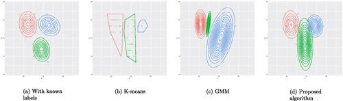
Table 5 Confusion tables for the flea beetle data set using the three clustering algorithms.

		cluster	heikertingeri	heptapotamica	concinna
	K-means	1	30	3	0
		2	1	19	9
		3	0	0	12
	GMM	1	20	0	0
		2	10	0	0
		3	1	22	21
Proposed	algorithm	1	30	1	0
		2	1	21	5
		3	0	0	16

Table 6 Descriptive statistics for the three identified clusters by the used clustering algorithms.

	Cluster 1
	n	$\overline{x}$	$\overline{y}$	σ11	σ12	σ22
True labels	31	124.65	14.29	21.37	–0.33	1.22
K-means	34	124.88	13.94	20.55	–2.07	2.75
GMM	20	121.86	14.34	7.22	–0.166	1.20
Prop. alg.	31	124.52	14.23	19.02	–0.44	1.47
	Cluster 2
	n	$\overline{x}$	$\overline{y}$	σ11	σ12	σ22
True labels	22	138.27	10.09	17.16	–0.50	0.94
K-means	29	139.79	11.55	9.96	0.51	5.04
GMM	10	129.63	14.33	1.19	0.74	0.97
Prop. alg.	27	138.52	10.96	12.77	–0.54	3.81
	Cluster 3
	n	$\overline{x}$	$\overline{y}$	σ11	σ12	σ22
True labels	21	146.19	14.10	31.66	–0.97	0.79
K-means	12	150.08	13.83	10.08	0.94	0.70
GMM	44	141.87	12.07	39.51	6.82	4.72
Prop. alg.	16	148.50	14.00	14.50	–0.135	0.75

The first line of each tabular represents the corresponding values using the true label of each observation.

Table

	Accuracy	Kappa
K-means	0.92	0.88
GMM	0.89	0.84
New	0.93	0.89

The best values for each case are indicated in bold.

Table

	Accuracy	Kappa
K-means	0.85	0.77
GMM	0.82	0.74
New	0.88	0.81

The best values for each case are indicated in bold.

Table

	Accuracy	Kappa
K-means	0.78	0.71
GMM	0.71	0.61
New	0.81	0.75

The best values for each case are indicated in bold.

Table

	Accuracy	Kappa
K-means	0.78	0.71
GMM	0.71	0.61
New	0.80	0.74

The best values for each case are indicated in bold.