Exploring the impact of how criminals interact with cyber-networks—a mathematical modeling approach

Figures & data

Figure 1. Flow diagram for the dynamics of cybercrime depicting how people transition between compartments as individuals experience cybercrime.

Figure 2. Plots of the steady-state proportion of the network that is victimised when the criminals are external to the network, i.e. with ψ = 0. Model parameters used: ${\sigma }_2=2$, ${\sigma }_3=1$, ${\sigma }_{4y}={\sigma }_{4c}=2$, ${\sigma }_5=1$, p = 0.75. In (a) ${\sigma }_1=0.5$, in (b) α = 0.5.

Figure 3. Plots of the steady-state proportion of the network that is victimised when the criminals are internal to the network, i.e. with ψ = 1. The solid blue line is the value y_e whilst the red crosses are given by $y_e/(1-\psi c)$ which is the proportion of available population in the network that are victimised at steady state. Model parameters used: ${\sigma }_2=2$, ${\sigma }_3=1$, ${\sigma }_{4y}={\sigma }_{4c}=2$, ${\sigma }_5=1$, p = 0.75. In (a) $c_e=0.01$, in (b) α = 0.5.

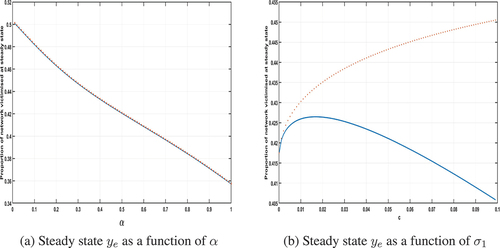
Figure 4. Plot of the proportion of available network members that are victimised at steady state as the rate of successful contact between susceptible and criminal individuals increases. Model parameters used: ${\sigma }_2=2$, ${\sigma }_3=1$, ${\sigma }_{4y}=2$, ${\sigma }_5=1$, p = 0.75, α = 0.5 and c = 0.02.