A new iterative computational scheme for solving second order (1 + 1) boundary value problems with non-homogeneous Dirichlet conditions

Figures & data

Figure 1. Graphs of heat equation. S₇ shows good convergence with the exact solution for (a) t = 0 and (b) t = 0.5.

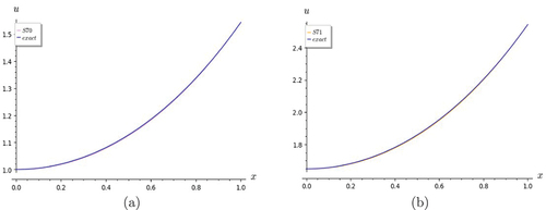
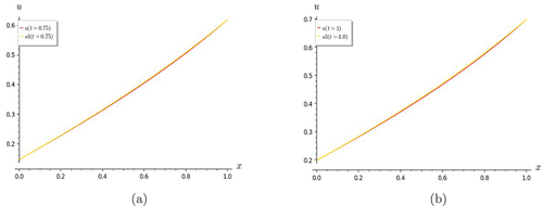
Figure 2. Graphs of heat equation. (a) shows S₇ converges well with exact solution for t = 1. (b) figure shows convergence of partial sums S₅, S₆ and S₇ for t = 0.

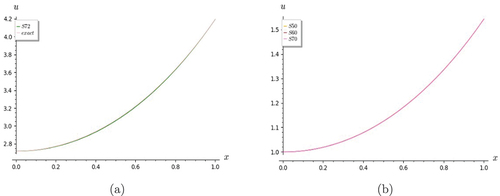
Figure 3. Graphs of heat equation. Figure shows convergence of partial sums for (a) $\mathit{t}=0.5,\mathit{and}(\mathit{b})\mathit{t}=1.$

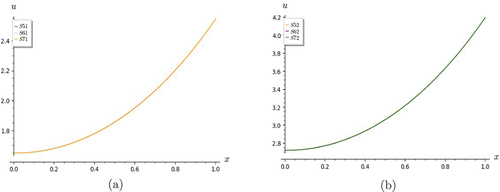
Table 1. Linear and homogeneous telegraph equation

x	t=0.0	t=0.5	t=1.0	t=2.0
0.0	0.00	0.00	0.00	0.00
	0.00	0.00	0.00	0.00
0.2	0.19866933	0.120499040	0.073086362	0.026886970
	0.19385399	0.117578388	0.071314897	0.026235284
0.5	0.479425538	0.290786288	0.176370799	0.064883190
	0.470121463	0.285143081	0.172948021	0.063624021
0.8	0.717356090	0.435098462	0.263900557	0.097083589
	0.710352389	0.430850503	0.261324039	0.096135741
1.0	0.841470984	0.510377951	0.309559875	0.113880714
	0.841770984	0.510377951	0.309559875	0.113880714

Figure 4. Graphs of Lin and Hom Telegraph Equation. S₇ shows a good rate of convergence with the exact solution for (a) t = 0 and (b) t = 0.5.

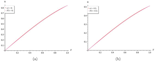
Figure 5. Graphs of Lin and Hom Telegraph Equation. (a) S₇ shows good convergence with the exact solution for t = 1.0; (b) the partial sums S₃, S₅ and S₇ are in good agreement for t = 0.

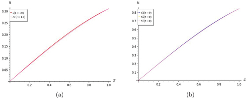
Figure 6. Graphs of Lin and Hom Telegraph Equation. The partial sums S₃, S₅ and S₇ are in good agreement for (a) t = 0.5 and (b) t= 1.

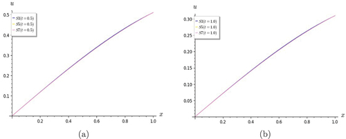
Figure 7. Graphs of Lin and Hom KG equation. S₇ shows good rate of convergence with the exact solution for (a) t = 0 and (b) t = 0.5.

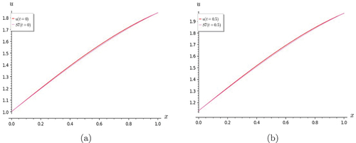
Figure 8. Graphs of Lin and Hom KG equation. (a) S₇ shows good convergence with the exact solution for t = 1.0; (b) the partial sums S₃, S₅ and S₇ are in good agreement for t = 0.

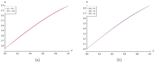
Figure 9. Graphs of Lin and homogeneous KG equation. The partial sums S₃, S₅ and S₇ are in good agreement for (a) t = 0.5 and (b) t = 1.

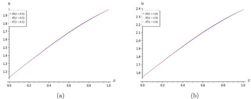
Figure 10. Graphs of Lin and non-homogeneous telegraph equation. Comparison of S₇ with the exact solution for (a) t = 0 and (b) t = 0.5.

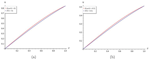
Figure 11. Graphs of Lin and non-homogeneous telegraph equation. S₇ shows good convergence with the exact solution for (a) t = 1.0 and (b) t = 2.0.

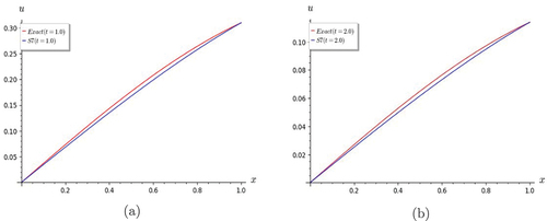
Figure 12. Graphs of Lin and non-homogeneous telegraph equation. S₇ shows good convergence with the exact solution for (a) t = 5.0. (b) The partial sums S₃, S₅ and S₇ converge when t = 0.

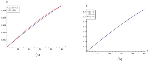
Figure 13. Graphs of Lin and non-homogeneous telegraph equation. The partial sums S₃, S₅ and S₇ converge at $(\mathit{a})\mathit{t}=0.5,(\mathit{b})\mathit{t}=1.0$.

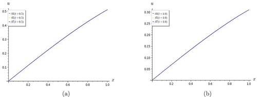
Figure 14. Graphs of nonlinear and non-homogeneous telegraph equation. S₄ converges very well with the exact solution when $(\mathit{a})\mathit{t}=0,(\mathit{b})0.5$.

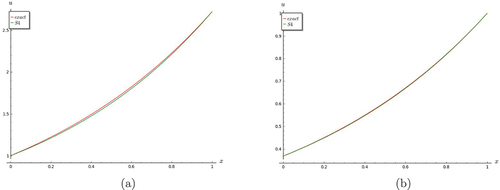
Figure 15. Graphs of nonlinear and non-homogeneous telegraph equation. (a) S₄ converges very well with the exact solution when t = 1.0. (b) shows that partial sums S₃ and S₄ converge when t = 0.

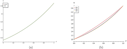
Figure 16. Graphs of nonlinear and non-homogeneous telegraph equation. Partial sums S₃ and S₄ converge when (a) t = 0.5 and (b) 1.0.

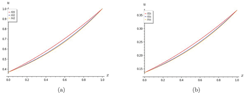
Figure 17. Graphs of Fisher equation. (a) S₃ deviates slightly from the exact solution for t = 0.25.(b) the convergence of S₃ to $\mathit{u}(\mathit{x},\mathit{t})$ is seen to be improving when $\mathit{t}\ge 0.5$, as found in the subsequent graphs for the equation.

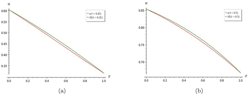
Figure 18. Graphs of Fisher equation. S₃ converges to $\mathit{u}(\mathit{x},\mathit{t})\mathit{at}(\mathit{a})\mathit{t}=0.75,(\mathit{b})\mathit{t}=1.0$.

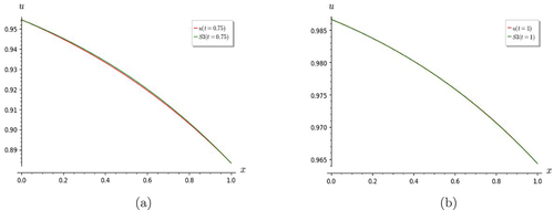
Figure 19. Graphs of Fisher equation. As t gets larger, the convergence of S₃ with $\mathit{u}(\mathit{x},\mathit{t})$ is seen to improve at (a) t=2, and (b) t=5.

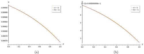
Figure 20. Fishers Eqn.-graphs of Fisher equation showing that S₃ converges to S₄ at (a) t=0.5, and (b) t=1.

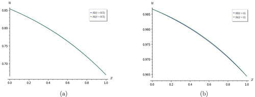
Figure 21. Graphs of nonlinear KG equation. (a) and (b) S₃ converges to $\mathit{u}(\mathit{x},\mathit{t})$ at (a) t=0 and (b) t=0.5, respectively.

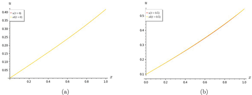
Figure 22. Graphs of nonlinear KG equation. (a) and (b) S₃ converges to $\mathit{u}(\mathit{x},\mathit{t})$ at t=0.75 and t=1.0, respectively.

Data availability statement

No data were used to support the study.