Layer adapted finite element method for two-parameter singularly perturbed delay parabolic problems

Figures & data

Figure 1. Global numerical solution indices refers to local nodes of arbitrary finite element $[x_{\mathit{i}},x_{\mathit{i}+1}]\times [t_{\mathit{j}},t_{\mathit{j}+1}]$.

Figure 2. Global numerical solution indices refers to local nodes of arbitrary finite element $[x_{\mathit{i}},x_{\mathit{i}+1}]\times [t_{\mathit{j}},t_{\mathit{j}+1}]$ after double split of the spatial and temporal finite elements.

Figure 3. Graphs of the FE solution of example 5.1 for $32\times 32$ mesh and double mesh grid with parameters $\mathit{\epsilon }={10}^{-10}$ and $\mathit{\mu }={10}^{-20}.$.

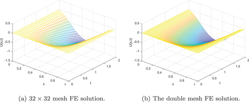
Figure 4. The graph of element-wise absolute maximum error of the FE solution in example 5.1 for $32\times 32$ mesh when the parameters $\mathit{\epsilon }={10}^{-10}$ and $\mathit{\mu }={10}^{-20}.$.

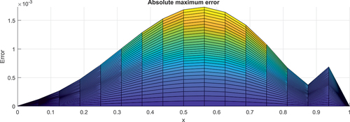
Figure 5. The graph of element-wise absolute maximum error of the FE solution in example 5.1 for $64\times 64$ mesh when the parameters $\mathit{\epsilon }={10}^{-10}$ and $\mathit{\mu }={10}^{-20}.$.

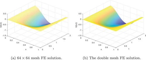
Figure 6. The graph of element-wise absolute maximum error of the FE solution in example 5.1 for $64\times 64$ mesh when the parameters $\mathit{\epsilon }={10}^{-10}$ and $\mathit{\mu }={10}^{-20}.$.

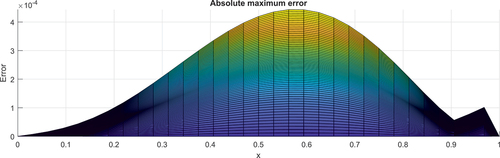
Figure 7. Graphs of the FE solution of example 5.2 for $32\times 32$ mesh and double mesh grid with parameters $\mathit{\epsilon }={10}^{-10}$ and $\mathit{\mu }={10}^{-20}.$.

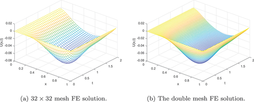
Figure 8. The graph of element-wise absolute maximum error of the FE solution in example 5.2 for $32\times 32$ mesh when the parameters $\mathit{\epsilon }={10}^{-10}$ and $\mathit{\mu }={10}^{-20}$.

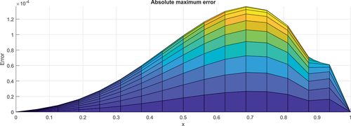
Figure 9. Graphs of the FE solution of example 5.2 for 64 × 64 mesh and double mesh grid with parameters ε = 10 − 10 and μ = 10 − 20.

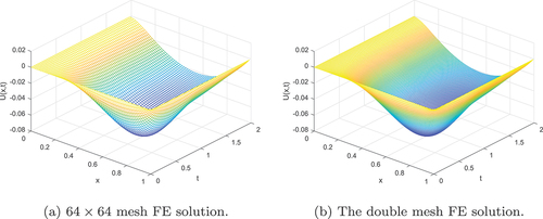
Figure 10. The graph of element-wise absolute maximum error of the FE solution in example 5.2 for 64 × 64 mesh when the parameters ε = 10 − 10 and μ = 10 − 20.

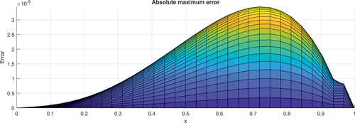
Table 1. Error estimate and convergence rate of example 5.1, for $\mathit{\epsilon }={10}^{-10}$

$\mathit{\mu }\downarrow$		N = 16	32	64	128	256	512
		M = 16	32	64	128	256	512
10^−6	$E_{\epsilon ,\mu }^{N,M}$	6.6767e-03	1.7327e-03	4.4312e-04	1.1309e-04	2.8711e-05	7.2680e-06
	$R_{\epsilon ,\mu }^{N,M}$	1.9461	1.9673	1.9702	1.9778	1.9819
10^−8	$E_{\epsilon ,\mu }^{N,M}$	6.6769e-03	1.7328e-03	4.4313e-04	1.1310e-04	2.8712e-05	7.2681e-06
	$R_{\epsilon ,\mu }^{N,M}$	1.9461	1.9673	1.9701	1.9779	1.9820
⋮	⋮	⋮	⋮	⋮	⋮	⋮	⋮
10^−18	$E_{\epsilon ,\mu }^{N,M}$	6.6769e-03	1.7328e-03	4.4313e-04	1.1310e-04	2.8712e-05	7.2681e-06
	$R_{\epsilon ,\mu }^{N,M}$	1.9461	1.9673	1.9701	1.9779	1.9820
10^−20	$E_{\epsilon ,\mu }^{N,M}$	6.6769e-03	1.7328e-03	4.4313e-04	1.1310e-04	2.8712e-05	7.2681e-06
	$R_{\epsilon ,\mu }^{N,M}$	1.9461	1.9673	1.9701	1.9779	1.9820
	$E^{\mathit{N},\mathit{M}}$	6.6769e-03	1.7328e-03	4.4313e-04	1.1310e-04	2.8712e-05	7.2681e-06
	$R^{\mathit{N},\mathit{M}}$	1.9461	1.9673	1.9701	1.9779	1.9820

Table 2. Error estimate and convergence rate of example 5.1, for $\mathit{\mu }={10}^{-10}$

$\mathit{\epsilon }\downarrow$		N = 16	32	64	128	256	512
		M = 16	32	64	128	256	512
10^−18	$E_{\epsilon ,\mu }^{N,M}$	6.6831e-03	1.7347e-03	4.4377e-04	1.1335e-04	2.8789e-05	7.2902e-06
	$R_{\epsilon ,\mu }^{N,M}$	1.9458	1.9668	1.9690	1.9772	1.9815
10^−20	$E_{\epsilon ,\mu }^{N,M}$	6.6831e-03	1.7347e-03	4.4377e-04	1.1335e-04	2.8789e-05	7.2902e-06
	$R_{\epsilon ,\mu }^{N,M}$	1.9458	1.9668	1.9690	1.9772	1.9815
⋮		⋮	⋮	⋮	⋮	⋮	⋮
10^−28	$E_{\epsilon ,\mu }^{N,M}$	6.6833e-03	1.7347e-03	4.4377e-04	1.1335e-04	2.8789e-05	7.2902e-06
	$R_{\epsilon ,\mu }^{N,M}$	1.9459	1.9668	1.9690	1.9772	1.9815
10^−30	$E_{\epsilon ,\mu }^{N,M}$	6.6833e-03	1.7347e-03	4.4377e-04	1.1335e-04	2.8789e-05	7.2902e-06
	$R_{\epsilon ,\mu }^{N,M}$	1.9459	1.9668	1.9690	1.9772	1.9815
	$E^{\mathit{N},\mathit{M}}$	6.6833e-03	1.7347e-03	4.4377e-04	1.1335e-04	2.8789e-05	7.2902e-06
	$R^{\mathit{N},\mathit{M}}$	1.9459	1.9668	1.9690	1.9772	1.9815

Table 3. Error estimate and convergence rate of example 5.2, for $\mathit{\epsilon }={10}^{-10}$

$\mathit{\mu }\downarrow$		N = 16	32	64	128	256	512
		M = 16	32	64	128	256	512
10^−6	$E_{\epsilon ,\mu }^{N,M}$	5.3629e-04	1.3641e-04	3.4453e-05	8.6810e-06	2.1805e-06	5.4584e-07
	$R_{\epsilon ,\mu }^{N,M}$	1.9751	1.9852	1.9887	1.9932	1.9981
10^−8	$E_{\epsilon ,\mu }^{N,M}$	5.3630e-04	1.3642e-04	3.4454e-05	8.6812e-06	2.1806e-06	5.4586e-07
	$R_{\epsilon ,\mu }^{N,M}$	1.9750	1.9853	1.9887	1.9932	1.9981
⋮		⋮	⋮	⋮	⋮	⋮	⋮
10^−18	$R_{\epsilon ,\mu }^{N,M}$	5.3630e-04	1.3642e-04	3.4454e-05	8.6812e-06	2.1806e-06	5.4586e-07
	$R_{\epsilon ,\mu }^{N,M}$	1.9750	1.9853	1.9887	1.9932	1.9981
10^−20	$E_{\epsilon ,\mu }^{N,M}$	5.3630e-04	1.3642e-04	3.4454e-05	8.6812e-06	2.1806e-06	5.4586e-07
	$R_{\epsilon ,\mu }^{N,M}$	1.9750	1.9853	1.9887	1.9932	1.9981
	$E^{\mathit{N},\mathit{M}}$	5.3630e-04	1.3642e-04	3.4454e-05	8.6812e-06	2.1806e-06	5.4586e-07
	$R_{\epsilon ,\mu }^{N,M}$	1.9750	1.9853	1.9887	1.9932	1.9981

Table 4. Error estimate and convergence rate of example 5.2, for $\mathit{\mu }={10}^{-10}$

$\mathit{\epsilon }\downarrow$		N = 16	32	64	128	256	512
		M = 16	32	64	128	256	512
10^−18	$E_{\epsilon ,\mu }^{N,M}$	5.3713e-04	1.3668e-04	3.4621e-05	8.6793e-06	2.1722e-06	5.4316e-07
	$R_{\epsilon ,\mu }^{N,M}$	1.9745	1.9811	1.9960	1.9984	1.9997
10^−20	$E_{\epsilon ,\mu }^{N,M}$	5.3713e-04	1.3668e-04	3.4621e-05	8.6793e-06	2.1722e-06	5.4316e-07
	$R_{\epsilon ,\mu }^{N,M}$	1.9745	1.9811	1.9960	1.9984	1.9997
⋮		⋮	⋮	⋮	⋮	⋮	⋮
10^−28	$E_{\epsilon ,\mu }^{N,M}$	5.3713e-04	1.3668e-04	3.4621e-05	8.6793e-06	2.1722e-06	5.4316e-07
	$R_{\epsilon ,\mu }^{N,M}$	1.9745	1.9811	1.9960	1.9984	1.9997
10^−30	$E_{\epsilon ,\mu }^{N,M}$	5.3713e-04	1.3668e-04	3.4621e-05	8.6793e-06	2.1722e-06	5.4316e-07
	$R_{\epsilon ,\mu }^{N,M}$	1.9745	1.9811	1.9960	1.9984	1.9997
	$E^{\mathit{N},\mathit{M}}$	5.3713e-04	1.3668e-04	3.4621e-05	8.6793e-06	2.1722e-06	5.4316e-07
	$R^{\mathit{N},\mathit{M}}$	1.9745	1.9811	1.9960	1.9984	1.9997

Figure 11. logarithmic scaled graphs of maximum error versus number of meshes:(a)Example 5.1, and (b) example 5.2.

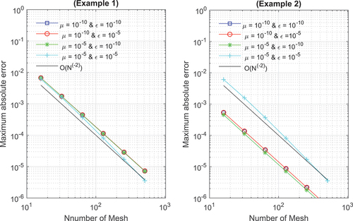
Table 5. Comparison of the error estimate $(E^{\mathit{N},\mathit{M}})$ and rate of convergence $(R^{\mathit{N},\mathit{M}})$ of example 5.1, for $\mathit{\epsilon }={10}^{-4}$ and $\mathit{\mu }={10}^{-9}$

	$\mathit{N}=$	32	64	128	256	512
Method	$\mathit{M}=$	8	16	32	64	128
(Kumar, et al., 2020)	$E^{\mathit{N},\mathit{M}}$	1.1100e-02	5.0838e-03	2.4640e-03	1.2162e-03	6.0457e-04
	$R^{\mathit{N},\mathit{M}}$	1.1265	1.0449	1.0185	1.0084
(Ayele et al., 2023),θ = 1	$E^{\mathit{N},\mathit{M}}$	5.4545e-03	2.8706e-03	1.4692e-03	7.4328e-04	3.7384e-04
	$R^{\mathit{N},\mathit{M}}$	0.9261	0.9663	0.9830	0.9915
(Ayele et al., 2023),$\mathit{\theta }=\frac{1}{2}$	$E^{\mathit{N},\mathit{M}}$	1.3176e-03	3.2988e-04	8.2475e-05	2.0620e-05	5.1550e-06
	$R^{\mathit{N},\mathit{M}}$	1.9979	1.9999	1.9999	2.0000
The Present	$E^{\mathit{N},\mathit{M}}$	5.4397e-04	1.1935e-04	2.8367e-05	7.0915e-06	1.7729e-06
	$R^{\mathit{N},\mathit{M}}$	2.1884	2.07291	2.0001	2.0000

Ayele, M. A., Tiruneh, A. A., & Derese, G. A. (2023). Fitted cubic spline scheme for two-parameter singularly perturbed time-delay parabolic problems. Results in Applied Mathematics, 18, 100361. https://doi.org/10.1016/j.rinam.2023.100361

 Google Scholar