
Figures & data
Figure 1. The digital twin is a representation of an actual object or process, monitored in real time, with the flow of information or data from the actual object or process to its twin. The twin itself represents a single instance of this object or process and can simulate its time evolution under normal or perturbed conditions. It offers facilities for basic user interaction and in this manner provides actionable knowledge, the added value of the twin. We consider these properties as essential to distinguish digital twins from other digital representations. The dotted arrow illustrates an optional feedback loop.
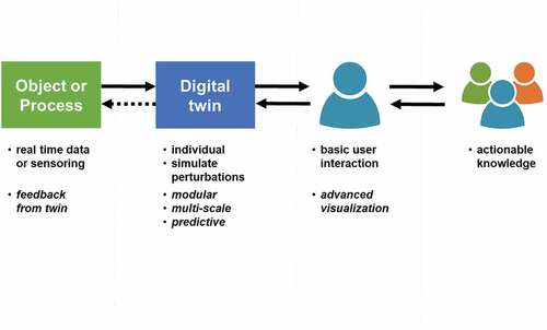
Figure 2. Screenshots from https://farmmaps.eu showing a simulation and forecast with the Tipstar potato model for a field near Wageningen, The Netherlands, in 2021. Simulated fresh tuber yield. The crop was planted on 15 April 2021 and the forecast was made on 14 July. From planting to 14 July, observed weather was used for the simulation. For the two weeks following 14 July, forecast weather was used. From 1 August, a stochastic simulation using 30 years of historic weather was performed, thus from 1 August the line becomes a plume.
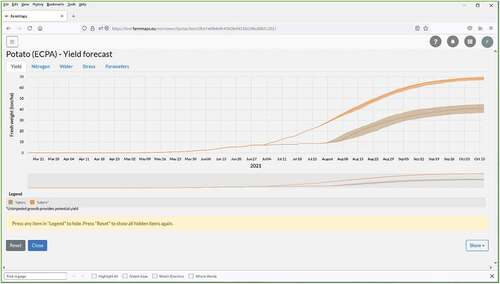
Figure 3. Same as but for simulated reduction of crop growth due to water-stress and N-stress. It shows that the crop is running out of N around the time of the forecast. At this point, the crop still looks healthy, and while the farmer cannot observe problems the model predicts these will occur soon.
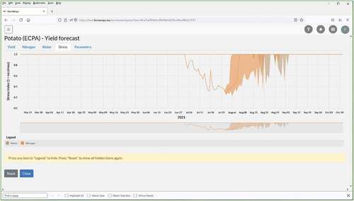
Figure 4. Simulation of potato growth with EnKF and Tipstar for Leaf Area Index (a) and for Tuber dry matter yield (b). The dashed red line shows the default simulation for this field. An ensemble of simulations (n = 50) is represented by grey-dotted lines; the ensemble median is shown with a solid black line. The filled square symbols show the LAI observations based on Sentinel-II imagery which were used to update the ensemble, and destructively measured tuber weights, for (a) and (b), respectively.
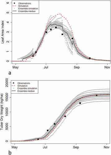
Figure 5. Variation in the EnKF simulation created with a parameter that influences LAI at emergence (a) and with a parameter that affects the lifespan of leaves (b).
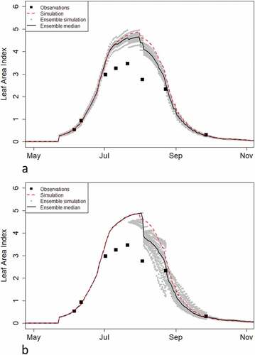
Figure 6. The role of decision support in greenhouse operational management. Two control loops are shown: a low-level management loop (with a low-level controller) with input consisting of settings and setpoints provided by the grower, and a high-level loop, in which a grower determines those settings and setpoints based on sensor information, forecasts and automated decision support (observation, prediction or control advice). Source photo: https://european-seed.com.
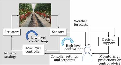
Figure 7. Role of the digital twin in decision support. Monitoring: the current state is estimated with an observer algorithm that employs the digital twin, together with sensor measurements. Prediction: the digital twin predicts the evolution of the state over a given time horizon. Control: using the current state estimation, together with the predictions of the digital twin, a control algorithm calculates the future control signals that optimize the operational management loop.
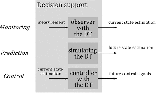
Figure 8. Simulated tomato plant growth in a virtual greenhouse environment. Visualisation created by Katarina Streit.
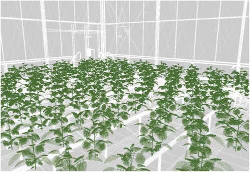
Table 1. Summarized findings of the three case studies.