Dynamic response analysis of fractional order RLC_α circuit and its order dependent oscillation criterion

Figures & data

Figure 1. RLC${}_{\alpha }$ circuit.

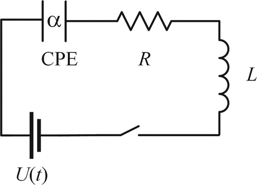
Figure 2. Integration contour in the 1st Riemann sheet.

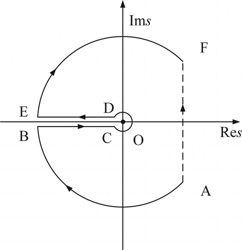
Figure 3. The curves of function $I(t)$ of different order when $R=1\mathrm{\Omega },L=1H,C=1F,E=5V.$

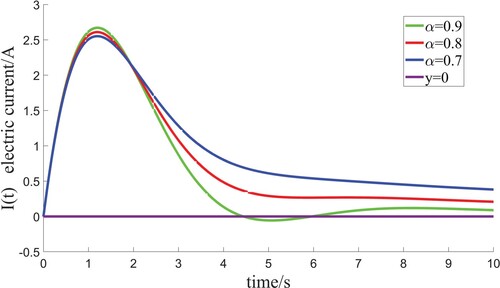
Figure 4. These graphs are for a critical damping case when R=1.08, L=1H, C=1F, E=1V.

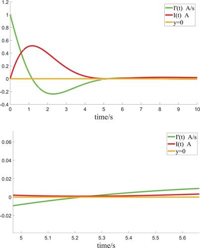
Figure 5. RC${}_{\alpha }$ series circuit.

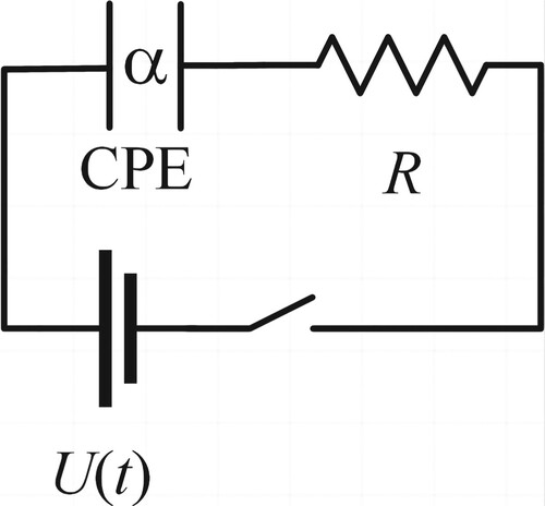
Figure 6. This graph corresponds to the impulse response g(t) with respect to the different order when $R=1\mathrm{\Omega },C=1F$. Method1 corresponds to the complex path integral method and method2 corresponds to Mittag–Leffler function series method.

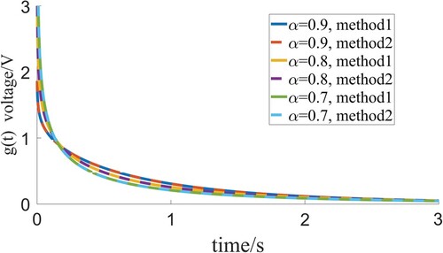
Figure 7. This graph is for the unit-step response $U_c(t)$ of different order when $R=5\mathrm{\Omega },C=1F$.

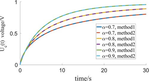
Figure 8. The dotted line corresponds to the solution using the inverse integral formula, chain line is for the solution using the Mittag–Leffler function.

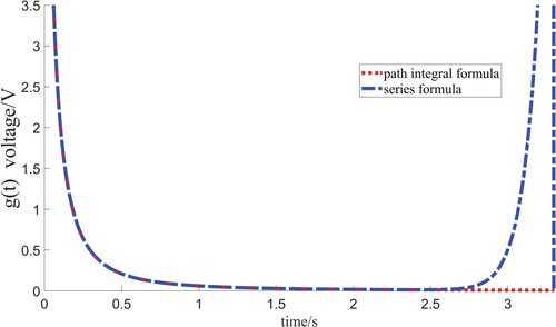
Figure 9. The critical damping phenomena of different order α with corresponding R when L=1000000H, C=0.01F, E=1V.

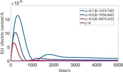
Figure 10. The critical damping phenomena of different order α with corresponding R when L=1000000H, C=0.001F, E=1V.

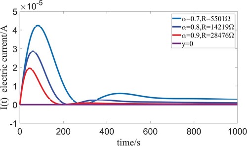
Figure 11. The critical damping phenomena of different order α with corresponding R when L=1000H, C=0.1F, E=1V.

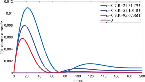
Figure 12. The damping phenomena of different resistors when α=0.9, L= 1000000H, C=0.1F, E=1V.

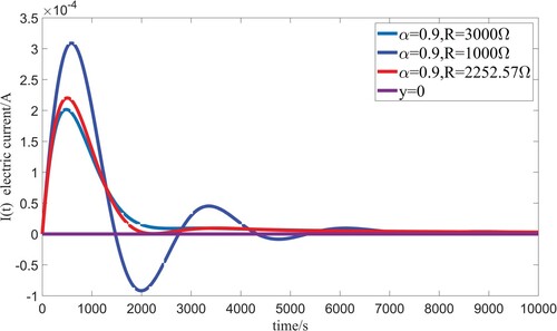
Table 1. The experimental data.

α	L(H)	C(F)	R(Ω)	λ	$t_1$(s)	$I(t_1)(A)$	$I^{\mathrm{\prime }}(t_1)(A/s)$
0.7	${10}^6$	0.01	1419.74	0.32	1123	$1.405\times {10}^{-6}$	$2.473\times {10}^{-11}$
0.8	${10}^6$	0.01	3956.60	0.66	818.5	$-3.15\times {10}^{-7}$	$4.451\times {10}^{-11}$
0.9	${10}^6$	0.01	8475.41	1.08	664.6	$2.261\times {10}^{-7}$	$1.175\times {10}^{-11}$
0.7	${10}^6$	0.001	5501	0.32	288.7	$8.872\times {10}^{-8}$	$3.941\times {10}^{-10}$
0.8	${10}^6$	0.001	14219	0.66	228.1	$-3.63\times {10}^{-8}$	$5.542\times {10}^{-10}$
0.9	${10}^6$	0.001	28476	1.08	198.1	$5.477\times {10}^{-8}$	$1.31\times {10}^{-10}$
0.7	${10}^3$	0.1	21.3147	0.32	74.43	$1.331\times {10}^{-5}$	$6.222\times {10}^{-9}$
0.8	${10}^3$	0.1	51.1014	0.66	63.63	$-1.06\times {10}^{-5}$	$2.134\times {10}^{-9}$
0.9	${10}^3$	0.1	95.6736	1.08	58.94	$9.873\times {10}^{-6}$	$3.644\times {10}^{-8}$

Table 2. The values of λ with respect to different fractional orders α.

α	0.7	0.8	0.9	1
λ	0.32	0.66	1.08	2