A hybrid method for an inverse scattering problem related to cylindrical bodies buried in a half-space

Figures & data

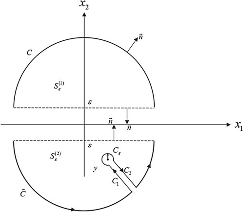
Figure 1. Geometry of the problem.

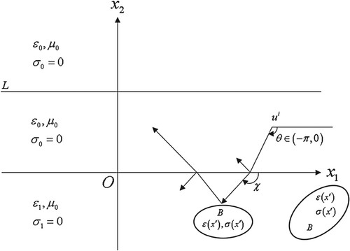
Figure 2. The degenerated regularity strip and branch cut in the complex $v$-plane.

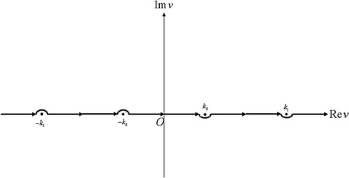
Figure 3. A layered region in the lower half-space ($y_2<0$).

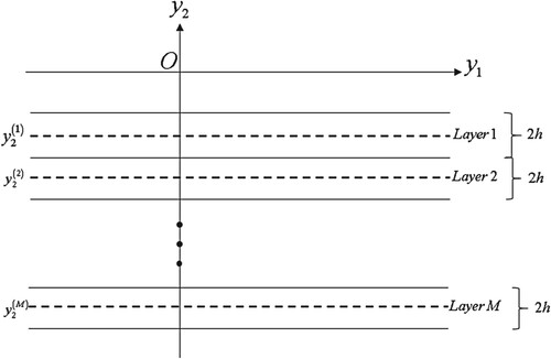
Figure 4. (a) The variation of the basis function ${\varphi }_0\left(y_1\right)$ and its support, (b) The Fourier transform variation of ${\varphi }_0\left(y_1\right)$ and its duration.

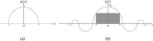
Figure 5. The variation of the basis functions ${\varphi }_n\left(y_1\right)$.

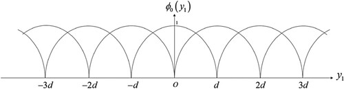
Figure 6. The geometries and the parameters for the illustrative examples. (a) Single cross-sectional case for $B$, (b) Case of several disjoint parts for $B$.

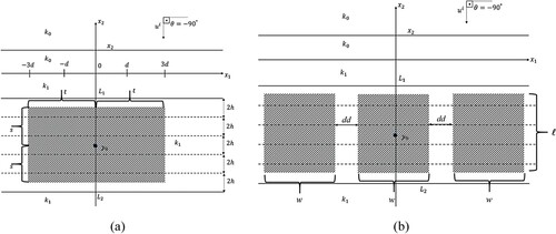
Figure 7. The computed and exact values of the object function $\upsilon \left(x^{\mathrm{\prime }}\right)$ for the case where the body$D$is completely out of the region $y_2\in \left(L_2,L_1\right)$. (a) Computed solution, (b) Exact solution.

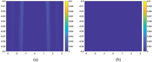
Figure 8. The computed and exact values of the object function $\upsilon \left(x^{\mathrm{\prime }}\right)$ for the case where a half of the body $D$ is in the region $y_2\in \left(L_2,L_1\right)$. (a) Computed solution, (b) Exact solution.

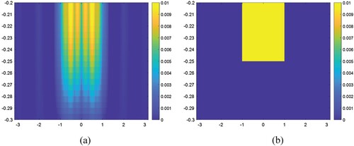
Figure 9. The computed and exact values of the object function $\upsilon \left(x^{\mathrm{\prime }}\right)$ for the case where the body D is completely in the region $y_2\in \left(L_2,L_1\right)$.

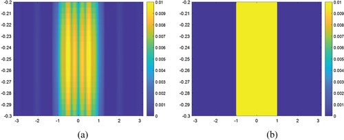
Figure 10. The computed and exact values of the object function $\upsilon \left(x^{\mathrm{\prime }}\right)$ for the case where the cross-section $B$ consists of two disjoint parts. (a) Computed solution, (b) Exact solution.

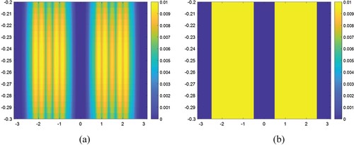
Figure 11. The computed and exact values of the object function $\upsilon \left(x^{\mathrm{\prime }}\right)$ for the case of diagonally overlapped disjoint parts of $B$. (a) Computed solution, (b) Exact solution.

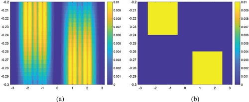
Figure 12. The computed and exact values of the object function $\upsilon \left(x^{\mathrm{\prime }}\right)$ for the case where the cross-section $B$ consists of three successive disjoint parts. (a) Computed solution, (b) Exact solution.

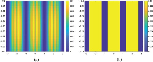
Figure 13. The computed and exact values of the object function $\upsilon \left(x^{\mathrm{\prime }}\right)$ for the case of full overlapped disjoint parts of $B$. (a) Computed solution, (b) Exact solution.

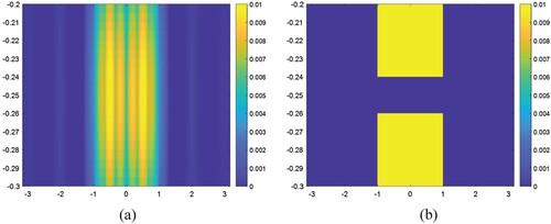
Figure 14. The computed results of the object functions related to different values of $d$. (a) $d={\lambda }_0/5$, (b) $d={\lambda }_0/6$, (c) $d={\lambda }_0/7$.

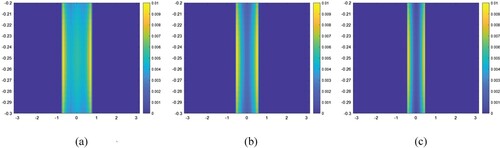
Figure 15. The computed results for the non-regularized situation. (a) Single cross-sectional case, (b)Triple cross-sectional case.

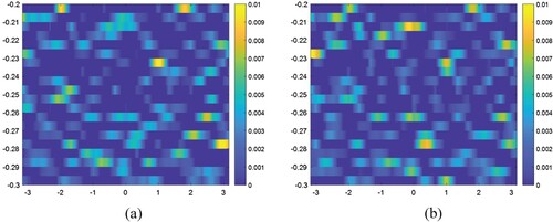
Figure 16. The computed and exact solutions of the object function $\upsilon \left(x^{\mathrm{\prime }}\right)$ considered as an illustrative in [32]. (a) Computed solution, (b) Exact solution

Figure 17. The computed and exact solutions of the object function $\upsilon \left(x^{\mathrm{\prime }}\right)$ considered as an illustrative in [31]. (a) Computed solution, (b) Exact solution.

Figure A1. The region $S_{ϵ}$ and its contour lines.

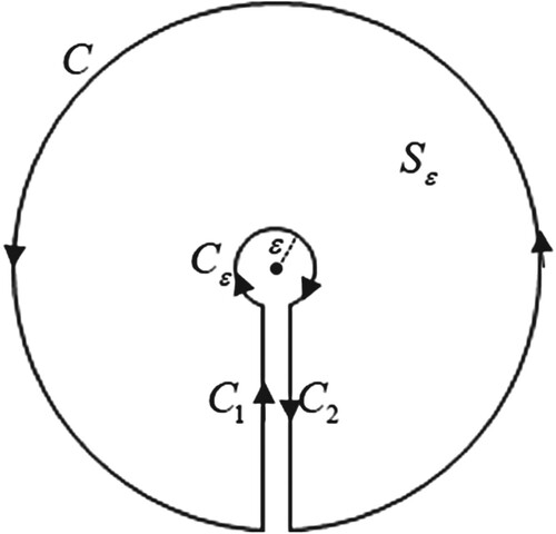
Figure A2. The regions and their contour lines for the two-part space case.

Alkumru A, Akduman I. Imaging of cylindrical bodies buried in a layered half-space bounded by an impedance plane. AEU Archiv für Elektronik und Übertragungstechnik. 1998;52(1):9–16.

 Google Scholar

Akduman I, Alkumru A. A generalized ART algorithm for inverse scattering problems related to buried cylindrical bodies. Inverse Prob. 1995;11(6):1125. doi:10.1088/0266-5611/11/6/001

 Web of Science ®Google Scholar