Phase-insensitive versus phase-sensitive ultrasound absorption tomography in the frequency domain

Figures & data

Table 1. Definitions for symbols used throughout this paper.

Symbol	Definition
χ, $\mathit{x}$	spatial domain, and spatial variable $\mathit{x}\in \chi$
${\chi }_{\theta ,m}\subset \chi$	spatial support of mth sensor at angle θ
$\omega ,\mathrm{\Omega }$	source frequency, set of source frequencies
$\theta ,\mathrm{\Theta }$	array rotation angle, set of array rotation angles
$S_{\omega \theta ,n}$	nth point source for frequency ω at angle θ
${\mathcal{L}}_{\omega }$	Helmholtz operator for source frequency ω
$\mathcal{M}$	pointwise field transformation based on sensor type
${\mathcal{I}}_{\theta ,m}$	measurement sampling operator for mth sensor at angle θ
${\mathit{y}}^{\mathcal{M}},y_{\omega \theta ,nm}^{\mathcal{M}}$	modelled data and its components for sensor type $\mathcal{M}$
${\mathit{g}}^{\mathcal{M}}$	measured data for sensor type $\mathcal{M}$
$\mathit{ϵ}$, ${ϵ}_i$	random noise vector and its components
$\tau ,\alpha$	dimensionless and dimensional absorption distributions
${\tau }_0$	modelled dimensionless absorption distribution
c	sound speed of medium
P	complex-valued pressure field
η	regularization parameter
$L_x,L_y$	pixel dimensions of simulation domain in x and y directions
${\mathbf{A}}_{\mathcal{M}},{\mathit{b}}^{\mathcal{M}}$	augmented forward matrix and data vector for sensor type $\mathcal{M}$
$F_{\mathcal{M}}:L^2\left(\chi \right)\to Y$	forward mapping from solution space $L^2\left(\chi \right)$ to data space Y, for sensor type given by $\mathcal{M}$
${\mathbf{J}}_{F_{\mathcal{M}}}{|}_{{\tau }_0},{\mathbf{J}}_{F_{\mathcal{M}}}{|}_{{\tau }_0}(i,\mathit{x})$, $({\mathbf{J}}_{F_{\mathcal{M}}}{|}_{{\tau }_0}{)}_{ij}$	Jacobian operator of $F_{\mathcal{M}}$ at ${\tau }_0$, its discrete-continuous components, and discretized components
$f_{\left\{i\right\}}\left(\right\{\mathit{z}\};\{a\left\}\right)$	function f with variables $\left\{\mathit{z}\right\}$, experimental parameters $\left\{i\right\}$, and medium parameters $\left\{a\right\}$

Figure 1. Parallel array source and sensor geometry where for a rotation of θ the mth sensor occupies a region ${\chi }_{\theta ,m}\subset \chi ={\mathbb{R}}^2$. Each of the M sensors in the array has a diameter of d, and is located at a distance D from the source array which consists of N point sources with continuous-wave signals defined by $S_{\omega \theta ,n}$ for the nth source.

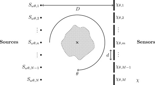
Figure 2. The true absorption difference profile, $\mathrm{\Delta }\tau =\tau -{\tau }_0$, that we wish to reconstruct. Region of interest for contrast analysis is indicated by the dashed red line box with the edge of the square-shaped absorption target acting as the mid-line. The parallel array with 10 point sources (white circles on the left) and 10 line sensors with $1\text{mm}$ diameter (white lines on the right) are shown for the zero rotation case, $\mathrm{\Delta }\theta =0^{\circ }$.

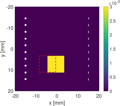
Table 2. Model parameters used for simulations.

Parameter (units)	Value(s)
Source frequency $\omega /2\pi$ (MHz)	1.5, 1.75, 2, 2.25, 2.5
Diameter of sensor d (mm)	1, 5
Rotation increment $\mathrm{\Delta }\theta$ (degrees)	7.5, 15, 30, 60
Source amplitude (Pa)	1
Source – sensor array separation D (mm)	30
Source array length (mm)	30
Sensor array length (mm)	30
Domain spatial dimensions x, y (mm)	40, 40
Domain pixel dimensions $L_x,L_y$ (pixels)	256, 256
Domain spatial increment dx = dy (mm)	0.15625
PML pixel width (pixels)	5

Figure 3. Reconstructions for PS and PI sensor types with 3 angles, 1 frequency ($\mathrm{\Omega }/\text{MHz}=\left\{2\right\}$), and $d=5\text{mm}$ sensors. (a) PS reconstruction with 0% noise. (b) PI reconstruction with 0% noise. (c) PS reconstruction with 1% noise. (d) PI reconstruction with 1% noise.

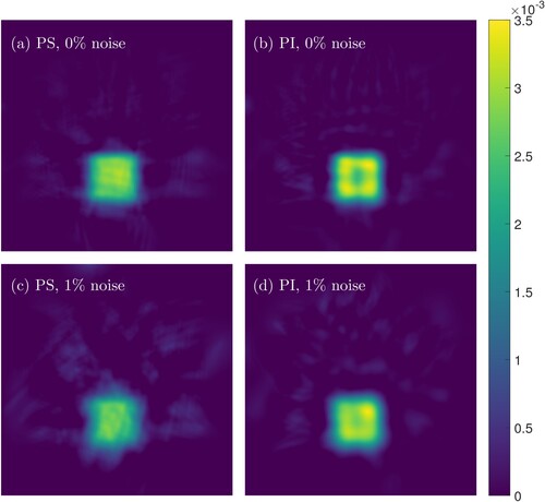
Figure 4. Reconstructions for PS and PI sensor types with 24 angles, 5 frequencies ($\mathrm{\Omega }/\text{MHz}=\{1.5,1.75,2,2.25,2.5\}$), and $d=1\text{mm}$ sensors. (a) PS reconstruction with 0% noise. (b) PI reconstruction with 0% noise. (c) PS reconstruction with 1% noise. (d) PI reconstruction with 1% noise.

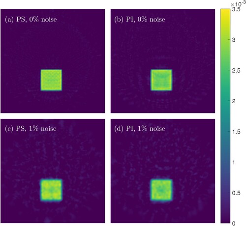
Figure 5. Contrast analysis and error curves for $5\text{mm}$ sensors. The plots on the left column show quantities for single-frequency reconstructions, whereas the right column shows the same quantities for 5-frequency reconstructions. (a)–(b) show the MTF FWHM, (c)–(d) show the maximum normalized contrasts, and (e)–(f) show the relative errors. The solid curves correspond to PS reconstructions whereas the dashed curves correspond to the PI reconstructions. The markers along the curves correspond to the noise-free (l) and noisy (♦) cases. (a) MTF FWHM, $|\mathrm{\Omega }|=1$, (b) MTF FWHM, $|\mathrm{\Omega }|=5$, (c) $C_{\mathrm{m}\mathrm{a}\mathrm{x}}$, $|\mathrm{\Omega }|=1$, (d) $C_{\mathrm{m}\mathrm{a}\mathrm{x}}$, $|\mathrm{\Omega }|=5$, (e) RE, $|\mathrm{\Omega }|=1$ and (f)RE, $|\mathrm{\Omega }|=5$.

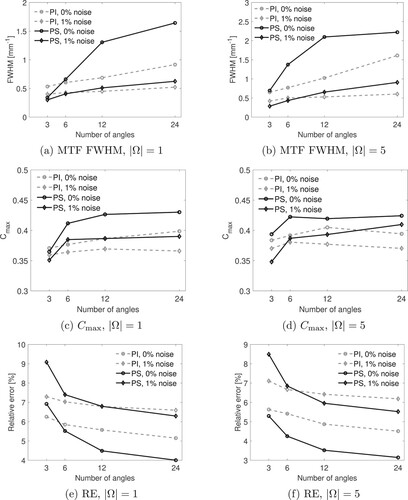
Figure 6. Contrast analysis and error curves for $1\text{mm}$ sensors. The plots on the left column show quantities for single frequency reconstructions, whereas the right column shows the same quantities for 5-frequency reconstructions. (a)–(b) show the MTF FWHM, (c)–(d) show the maximum normalized contrasts, and (e)–(f) show the relative errors. The solid curves correspond to PS reconstructions whereas the dashed curves correspond to the PI reconstructions. The markers along the curves correspond to the noise-free (l) and noisy (♦) cases. (a) MTF FWHM, $|\mathrm{\Omega }|=1$. (b) MTF FWHM, $|\mathrm{\Omega }|=5$. (c) $C_{\mathrm{m}\mathrm{a}\mathrm{x}}$, $|\mathrm{\Omega }|=1$. (d) $C_{\mathrm{m}\mathrm{a}\mathrm{x}}$, $|\mathrm{\Omega }|=5$. (e) RE, $|\mathrm{\Omega }|=1$ and (f)RE, $|\mathrm{\Omega }|=5$.

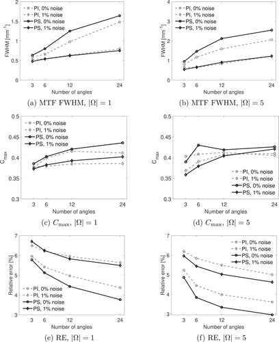
Figure A1. Profile for acoustic medium used for testing Jacobian robustness for sound speed heterogeneities. (a) Binary image of disk-shaped sound speed and square-shaped absorption perturbations in the acoustic medium and (b) Disk-shaped sound speed perturbation for the case of a sound speed deviation $\mathrm{\Delta }c=30$ [m/s] from the background value.

Figure A2. Relative ${\ell }_2$ error for reconstructions with increasing sound speed perturbation magnitude for a disk-shaped sound speed perturbation with a radius of $3.91\text{mm}$ (25 pixels). (a) 3 angles, 1 frequency and(b) 12 angles, 1 frequency

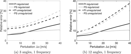
Figure A3. 3 angle minimum error reconstructions for the square-shaped absorption perturbation for varying magnitudes of the disk-shaped sound speed perturbation.

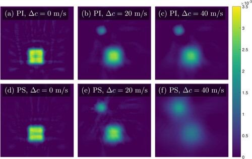
Figure A4. 12 angle minimum error reconstructions for the square-shaped absorption perturbation for varying magnitudes of the disk-shaped sound speed perturbation.

Figure A5. 3 angle unregularised reconstructions for the square-shaped absorption perturbation for varying magnitudes of the disk-shaped sound speed perturbation.

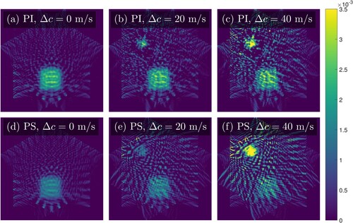
Figure A6. 12 angle unregularised reconstructions for the square-shaped absorption perturbation for varying magnitudes of the disk-shaped sound speed perturbation.

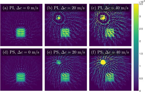
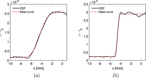
Figure A7. Error function f (red dashed line) fitted to the ensemble average of ESFs (solid black line) for the cases of (a) $d=5\text{mm}$ PS sensors with 3 angles, 1 frequency, and $1\mathrm{\%}$ noise, and (b) $d=1\text{mm}$ PS sensors with 24 angles, 5 frequencies, and $1\mathrm{\%}$ noise.