The complex dynamical behaviour of fractal-fractional forestry biomass system

Figures & data

Figure 1. A diagrammatic graph presentation of the forestry biomass relations of given the system is like as. In the flow diagram, $f\left(P\right)$ represents the function of forestry biomass (trees), which combines logistic growth and new plantation, described as $f\left(P\right)=\mathrm{rP}(1-\frac{P}{K})+\mathrm{\gamma P}$, $f_1(N,P)=r_{0}N(1-\frac{P}{K})$, $f_2(P,E)$ is the function of forestry biomass and industrial density through legal and illegal logging, $f_2(P,E)=d_1\mathrm{PE}+q_1\mathrm{PE}$ and $f_3(P,I)=\frac{\mathrm{\mu IP}}{K}.$ With the help of arrows and labels, the intensity and relationship between the compartments are marked.

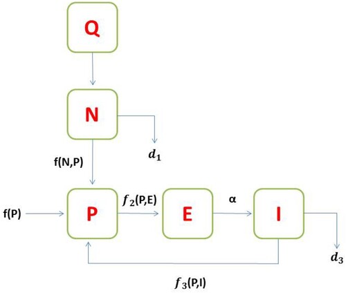
Table 1. Displays the parameter values in the following manner.

Parameters	Numerical values	Description
Q	4	Constant input rate of nutrients
β	0.7	Utilization rate of nutrients by forestry biomass
$d_1$	0.3	Washout rate of nutrients
r	0.2	Modified intrinsic growth rate of forestry biomass
$r_0$	0.01	Constant
K	70	Carrying capacity of forestry biomass
$q_1$	0.2	Harvesting rate of forestry biomass
γ	0.1	New plantation rate
$d_2$	0.03	Illegal logging of forestry biomass
p	0.35	Fixed price unit of forestry biomass
τ	0.25	Tax per unit of forestry biomass
c	0.08	Fixed cost per unit of effort expanded to harvest forestry biomass
α	0.03	Constant
μ	0.1	Maximum growth due to alternative industries
$d_3$	0.3	Reduction rate of industries

Figure 2. Numerical simulation of forestry biomass model (31(31) $\begin{array}{rl}{}^{\mathrm{FFP}}{}_{0+}{\mathfrak{D}}_t^{\psi ,\phi }N\left(t\right)& =Q-\text{β}P-d_{1}N,\\ {}^{\mathrm{FFP}}{}_{0+}{\mathfrak{D}}_t^{\psi ,\phi }P\left(t\right)& =r\left(N\right)P(1-\frac{P}{K})-q_1\mathrm{PE}-d_2\mathrm{PE}+\mathrm{\gamma P},\\ {}^{\mathrm{FFP}}{}_{0+}{\mathfrak{D}}_t^{\psi ,\phi }E\left(t\right)& =q_1(p-\tau )\mathrm{PE}+p{d}_2\mathrm{PE}-\mathrm{cE},\\ {}^{\mathrm{FFP}}{}_{0+}{\mathfrak{D}}_t^{\psi ,\phi }I\left(t\right)& =\mathrm{\alpha E}+\mathrm{\mu I}(1-\frac{P}{K})-d_{3}I.\end{array}$(31) ) at arbitrary values of ψ and φ. (a) Plot for Nutrient density N(t). (b) Plot for Forestry biomass P(t). (c) Plot for Efforts density E(t) and (d) Plot for Industrial density I(t).

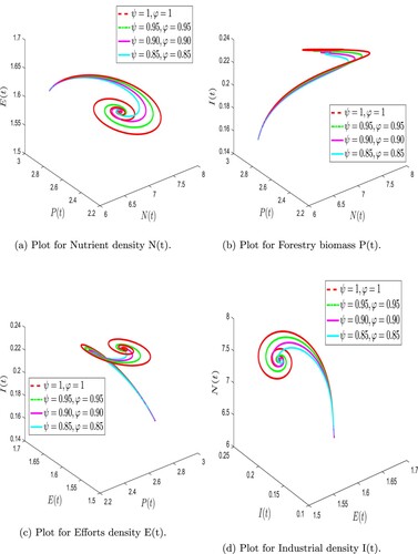
Figure 3. Numerical simulation of forestry biomass model (31(31) $\begin{array}{rl}{}^{\mathrm{FFP}}{}_{0+}{\mathfrak{D}}_t^{\psi ,\phi }N\left(t\right)& =Q-\text{β}P-d_{1}N,\\ {}^{\mathrm{FFP}}{}_{0+}{\mathfrak{D}}_t^{\psi ,\phi }P\left(t\right)& =r\left(N\right)P(1-\frac{P}{K})-q_1\mathrm{PE}-d_2\mathrm{PE}+\mathrm{\gamma P},\\ {}^{\mathrm{FFP}}{}_{0+}{\mathfrak{D}}_t^{\psi ,\phi }E\left(t\right)& =q_1(p-\tau )\mathrm{PE}+p{d}_2\mathrm{PE}-\mathrm{cE},\\ {}^{\mathrm{FFP}}{}_{0+}{\mathfrak{D}}_t^{\psi ,\phi }I\left(t\right)& =\mathrm{\alpha E}+\mathrm{\mu I}(1-\frac{P}{K})-d_{3}I.\end{array}$(31) ) at arbitrary values of ψ and φ. (a) Plot for Nutrient density N(t). (b) Plot for Forestry biomass P(t). (c) Plot for Efforts density E(t) and (d) Plot for Industrial density I(t).

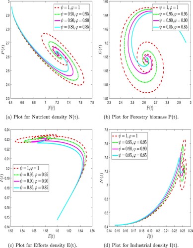
Figure 4. Numerical simulation of forestry biomass model (31(31) $\begin{array}{rl}{}^{\mathrm{FFP}}{}_{0+}{\mathfrak{D}}_t^{\psi ,\phi }N\left(t\right)& =Q-\text{β}P-d_{1}N,\\ {}^{\mathrm{FFP}}{}_{0+}{\mathfrak{D}}_t^{\psi ,\phi }P\left(t\right)& =r\left(N\right)P(1-\frac{P}{K})-q_1\mathrm{PE}-d_2\mathrm{PE}+\mathrm{\gamma P},\\ {}^{\mathrm{FFP}}{}_{0+}{\mathfrak{D}}_t^{\psi ,\phi }E\left(t\right)& =q_1(p-\tau )\mathrm{PE}+p{d}_2\mathrm{PE}-\mathrm{cE},\\ {}^{\mathrm{FFP}}{}_{0+}{\mathfrak{D}}_t^{\psi ,\phi }I\left(t\right)& =\mathrm{\alpha E}+\mathrm{\mu I}(1-\frac{P}{K})-d_{3}I.\end{array}$(31) ) at arbitrary values of ψ and φ. (a) Plot for Nutrient density N(t). (b) Plot for Forestry biomass P(t). (c) Plot for Efforts density E(t) and (d) Plot for Industrial density I(t).

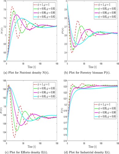
Figure 5. Numerical simulation of forestry biomass model (31(31) $\begin{array}{rl}{}^{\mathrm{FFP}}{}_{0+}{\mathfrak{D}}_t^{\psi ,\phi }N\left(t\right)& =Q-\text{β}P-d_{1}N,\\ {}^{\mathrm{FFP}}{}_{0+}{\mathfrak{D}}_t^{\psi ,\phi }P\left(t\right)& =r\left(N\right)P(1-\frac{P}{K})-q_1\mathrm{PE}-d_2\mathrm{PE}+\mathrm{\gamma P},\\ {}^{\mathrm{FFP}}{}_{0+}{\mathfrak{D}}_t^{\psi ,\phi }E\left(t\right)& =q_1(p-\tau )\mathrm{PE}+p{d}_2\mathrm{PE}-\mathrm{cE},\\ {}^{\mathrm{FFP}}{}_{0+}{\mathfrak{D}}_t^{\psi ,\phi }I\left(t\right)& =\mathrm{\alpha E}+\mathrm{\mu I}(1-\frac{P}{K})-d_{3}I.\end{array}$(31) ) at arbitrary values of ψ and fixed $\phi =1$. (a) Plot for Nutrient density N(t). (b) Plot for Forestry biomass P(t). (c) Plot for Efforts density E(t) and (d) Plot for Industrial density I(t).

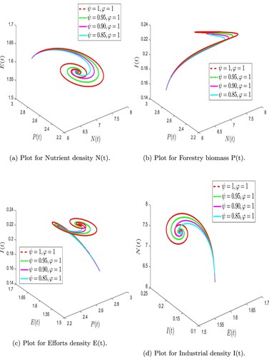
Figure 6. Numerical simulation of forestry biomass model (31(31) $\begin{array}{rl}{}^{\mathrm{FFP}}{}_{0+}{\mathfrak{D}}_t^{\psi ,\phi }N\left(t\right)& =Q-\text{β}P-d_{1}N,\\ {}^{\mathrm{FFP}}{}_{0+}{\mathfrak{D}}_t^{\psi ,\phi }P\left(t\right)& =r\left(N\right)P(1-\frac{P}{K})-q_1\mathrm{PE}-d_2\mathrm{PE}+\mathrm{\gamma P},\\ {}^{\mathrm{FFP}}{}_{0+}{\mathfrak{D}}_t^{\psi ,\phi }E\left(t\right)& =q_1(p-\tau )\mathrm{PE}+p{d}_2\mathrm{PE}-\mathrm{cE},\\ {}^{\mathrm{FFP}}{}_{0+}{\mathfrak{D}}_t^{\psi ,\phi }I\left(t\right)& =\mathrm{\alpha E}+\mathrm{\mu I}(1-\frac{P}{K})-d_{3}I.\end{array}$(31) ) at arbitrary values of ψ and fixed $\phi =1$. (a) Plot for Nutrient density N(t). (b) Plot for Forestry biomass P(t). (c)Plot for Efforts density E(t) and (d)Plot for Industrial density I(t).

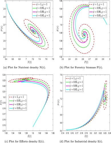
Figure 7. Numerical simulation of forestry biomass model (31(31) $\begin{array}{rl}{}^{\mathrm{FFP}}{}_{0+}{\mathfrak{D}}_t^{\psi ,\phi }N\left(t\right)& =Q-\text{β}P-d_{1}N,\\ {}^{\mathrm{FFP}}{}_{0+}{\mathfrak{D}}_t^{\psi ,\phi }P\left(t\right)& =r\left(N\right)P(1-\frac{P}{K})-q_1\mathrm{PE}-d_2\mathrm{PE}+\mathrm{\gamma P},\\ {}^{\mathrm{FFP}}{}_{0+}{\mathfrak{D}}_t^{\psi ,\phi }E\left(t\right)& =q_1(p-\tau )\mathrm{PE}+p{d}_2\mathrm{PE}-\mathrm{cE},\\ {}^{\mathrm{FFP}}{}_{0+}{\mathfrak{D}}_t^{\psi ,\phi }I\left(t\right)& =\mathrm{\alpha E}+\mathrm{\mu I}(1-\frac{P}{K})-d_{3}I.\end{array}$(31) ) at arbitrary values of ψ and fixed $\phi =1$. (a) Plot for Nutrient density N(t). (b) Plot for Forestry biomass P(t). (c) Plot for Efforts density E(t) and (d) Plot for Industrial density I(t).

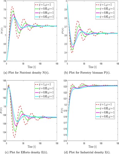
Figure 8. Numerical simulation of forestry biomass model (31(31) $\begin{array}{rl}{}^{\mathrm{FFP}}{}_{0+}{\mathfrak{D}}_t^{\psi ,\phi }N\left(t\right)& =Q-\text{β}P-d_{1}N,\\ {}^{\mathrm{FFP}}{}_{0+}{\mathfrak{D}}_t^{\psi ,\phi }P\left(t\right)& =r\left(N\right)P(1-\frac{P}{K})-q_1\mathrm{PE}-d_2\mathrm{PE}+\mathrm{\gamma P},\\ {}^{\mathrm{FFP}}{}_{0+}{\mathfrak{D}}_t^{\psi ,\phi }E\left(t\right)& =q_1(p-\tau )\mathrm{PE}+p{d}_2\mathrm{PE}-\mathrm{cE},\\ {}^{\mathrm{FFP}}{}_{0+}{\mathfrak{D}}_t^{\psi ,\phi }I\left(t\right)& =\mathrm{\alpha E}+\mathrm{\mu I}(1-\frac{P}{K})-d_{3}I.\end{array}$(31) ) at arbitrary values of φ and fixed $\psi =1$. (a) Plot for Nutrient density N(t). (b) Plot for Forestry biomass P(t). (c) Plot for Efforts density E(t) and (d) Plot for Industrial density I(t).

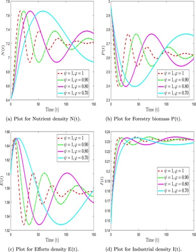
Figure 9. Numerical simulation of forestry biomass model (6(6) $\begin{array}{rl}{}^{\mathrm{FFE}}{}_{0+}{\mathfrak{D}}_t^{\psi ,\phi }N\left(t\right)& =Q-\text{β}P-d_{1}N,\\ {}^{\mathrm{FFE}}{}_{0+}{\mathfrak{D}}_t^{\psi ,\phi }P\left(t\right)& =r\left(N\right)P(1-\frac{P}{K})-q_1\mathrm{PE}-d_2\mathrm{PE}+\mathrm{\gamma P},\\ {}^{\mathrm{FFE}}{}_{0+}{\mathfrak{D}}_t^{\psi ,\phi }E\left(t\right)& =q_1(p-\tau )\mathrm{PE}+p{d}_2\mathrm{PE}-\mathrm{cE},\\ {}^{\mathrm{FFE}}{}_{0+}{\mathfrak{D}}_t^{\psi ,\phi }I\left(t\right)& =\mathrm{\alpha E}+\mathrm{\mu I}(1-\frac{P}{K})-d_{3}I,\end{array}$(6) ) at arbitrary values of ψ. (a) Plot for Nutrient density N(t). (b) Plot for Forestry biomass P(t). (c) Plot for Efforts density E(t) and (d) Plot for Industrial density I(t).

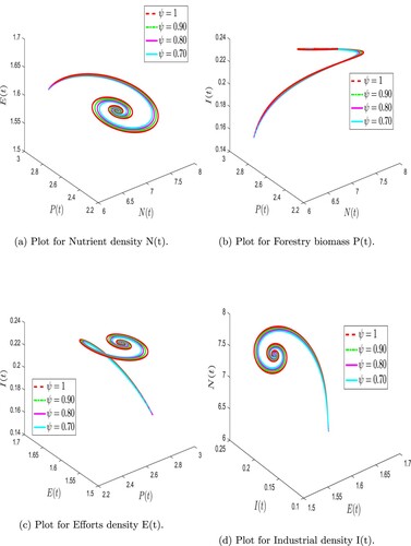
Figure 10. Numerical simulation of forestry biomass model (6(6) $\begin{array}{rl}{}^{\mathrm{FFE}}{}_{0+}{\mathfrak{D}}_t^{\psi ,\phi }N\left(t\right)& =Q-\text{β}P-d_{1}N,\\ {}^{\mathrm{FFE}}{}_{0+}{\mathfrak{D}}_t^{\psi ,\phi }P\left(t\right)& =r\left(N\right)P(1-\frac{P}{K})-q_1\mathrm{PE}-d_2\mathrm{PE}+\mathrm{\gamma P},\\ {}^{\mathrm{FFE}}{}_{0+}{\mathfrak{D}}_t^{\psi ,\phi }E\left(t\right)& =q_1(p-\tau )\mathrm{PE}+p{d}_2\mathrm{PE}-\mathrm{cE},\\ {}^{\mathrm{FFE}}{}_{0+}{\mathfrak{D}}_t^{\psi ,\phi }I\left(t\right)& =\mathrm{\alpha E}+\mathrm{\mu I}(1-\frac{P}{K})-d_{3}I,\end{array}$(6) ) at arbitrary values of ψ. (a) Plot for Nutrient density N(t). (b) Plot for Forestry biomass P(t). (c) Plot for Efforts density E(t) and (d) Plot for Industrial density I(t).

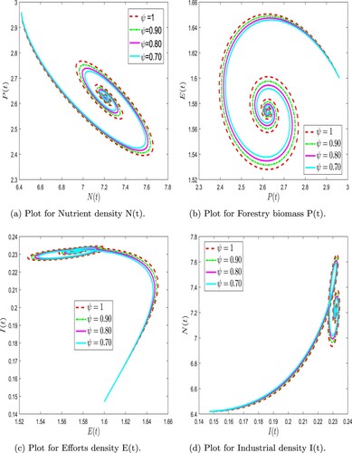
Figure 11. Numerical simulation of forestry biomass model (6(6) $\begin{array}{rl}{}^{\mathrm{FFE}}{}_{0+}{\mathfrak{D}}_t^{\psi ,\phi }N\left(t\right)& =Q-\text{β}P-d_{1}N,\\ {}^{\mathrm{FFE}}{}_{0+}{\mathfrak{D}}_t^{\psi ,\phi }P\left(t\right)& =r\left(N\right)P(1-\frac{P}{K})-q_1\mathrm{PE}-d_2\mathrm{PE}+\mathrm{\gamma P},\\ {}^{\mathrm{FFE}}{}_{0+}{\mathfrak{D}}_t^{\psi ,\phi }E\left(t\right)& =q_1(p-\tau )\mathrm{PE}+p{d}_2\mathrm{PE}-\mathrm{cE},\\ {}^{\mathrm{FFE}}{}_{0+}{\mathfrak{D}}_t^{\psi ,\phi }I\left(t\right)& =\mathrm{\alpha E}+\mathrm{\mu I}(1-\frac{P}{K})-d_{3}I,\end{array}$(6) ) at arbitrary values of ψ. (a) Plot for Nutrient density N(t). (b) Plot for Forestry biomass P(t). (c) Plot for Efforts density E(t) and (d) Plot for Industrial density I(t).

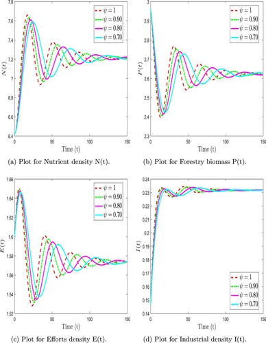
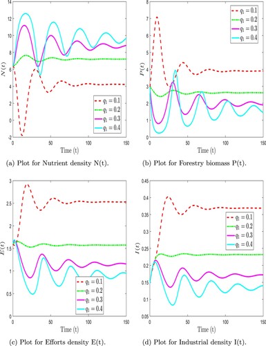
Figure 12. Numerical simulation of forestry biomass model (31(31) $\begin{array}{rl}{}^{\mathrm{FFP}}{}_{0+}{\mathfrak{D}}_t^{\psi ,\phi }N\left(t\right)& =Q-\text{β}P-d_{1}N,\\ {}^{\mathrm{FFP}}{}_{0+}{\mathfrak{D}}_t^{\psi ,\phi }P\left(t\right)& =r\left(N\right)P(1-\frac{P}{K})-q_1\mathrm{PE}-d_2\mathrm{PE}+\mathrm{\gamma P},\\ {}^{\mathrm{FFP}}{}_{0+}{\mathfrak{D}}_t^{\psi ,\phi }E\left(t\right)& =q_1(p-\tau )\mathrm{PE}+p{d}_2\mathrm{PE}-\mathrm{cE},\\ {}^{\mathrm{FFP}}{}_{0+}{\mathfrak{D}}_t^{\psi ,\phi }I\left(t\right)& =\mathrm{\alpha E}+\mathrm{\mu I}(1-\frac{P}{K})-d_{3}I.\end{array}$(31) ) at arbitrary values of $d_2$ with $\psi =0.99$. (a) Plot for Nutrient density N(t). (b) Plot for Forestry biomass P(t). (c) Plot for Efforts density E(t) and (d) Plot for Industrial density I(t).

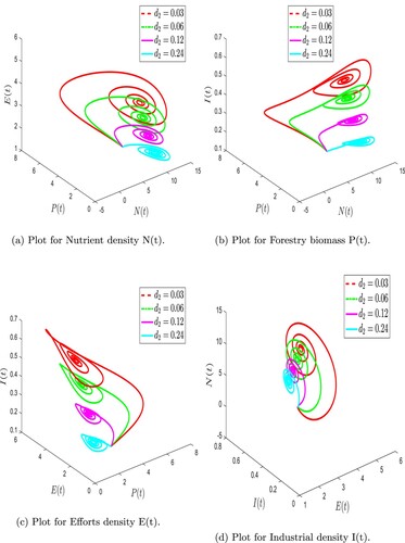
Figure 13. Numerical simulation of forestry biomass model (31(31) $\begin{array}{rl}{}^{\mathrm{FFP}}{}_{0+}{\mathfrak{D}}_t^{\psi ,\phi }N\left(t\right)& =Q-\text{β}P-d_{1}N,\\ {}^{\mathrm{FFP}}{}_{0+}{\mathfrak{D}}_t^{\psi ,\phi }P\left(t\right)& =r\left(N\right)P(1-\frac{P}{K})-q_1\mathrm{PE}-d_2\mathrm{PE}+\mathrm{\gamma P},\\ {}^{\mathrm{FFP}}{}_{0+}{\mathfrak{D}}_t^{\psi ,\phi }E\left(t\right)& =q_1(p-\tau )\mathrm{PE}+p{d}_2\mathrm{PE}-\mathrm{cE},\\ {}^{\mathrm{FFP}}{}_{0+}{\mathfrak{D}}_t^{\psi ,\phi }I\left(t\right)& =\mathrm{\alpha E}+\mathrm{\mu I}(1-\frac{P}{K})-d_{3}I.\end{array}$(31) ) at arbitrary values of $d_2$ with $\psi =0.99$. (a) Plot for Nutrient density N(t). (b) Plot for Forestry biomass P(t). (c) Plot for Efforts density E(t) and (d) Plot for Industrial density I(t).

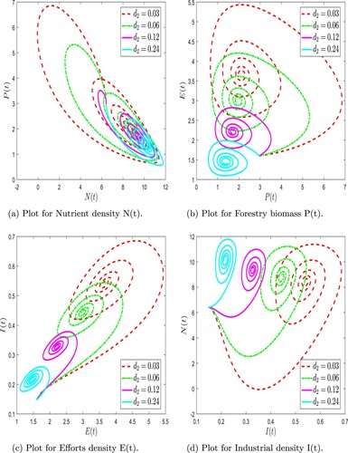
Figure 14. Numerical simulation of forestry biomass model (31(31) $\begin{array}{rl}{}^{\mathrm{FFP}}{}_{0+}{\mathfrak{D}}_t^{\psi ,\phi }N\left(t\right)& =Q-\text{β}P-d_{1}N,\\ {}^{\mathrm{FFP}}{}_{0+}{\mathfrak{D}}_t^{\psi ,\phi }P\left(t\right)& =r\left(N\right)P(1-\frac{P}{K})-q_1\mathrm{PE}-d_2\mathrm{PE}+\mathrm{\gamma P},\\ {}^{\mathrm{FFP}}{}_{0+}{\mathfrak{D}}_t^{\psi ,\phi }E\left(t\right)& =q_1(p-\tau )\mathrm{PE}+p{d}_2\mathrm{PE}-\mathrm{cE},\\ {}^{\mathrm{FFP}}{}_{0+}{\mathfrak{D}}_t^{\psi ,\phi }I\left(t\right)& =\mathrm{\alpha E}+\mathrm{\mu I}(1-\frac{P}{K})-d_{3}I.\end{array}$(31) ) at arbitrary values of $d_2$ with $\psi =0.99$. (a) Plot for Nutrient density N(t). (b) Plot for Forestry biomass P(t). (c) Plot for Efforts density E(t) and (d) Plot for Industrial density I(t).

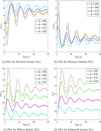
Figure 15. Numerical simulation of forestry biomass model (31(31) $\begin{array}{rl}{}^{\mathrm{FFP}}{}_{0+}{\mathfrak{D}}_t^{\psi ,\phi }N\left(t\right)& =Q-\text{β}P-d_{1}N,\\ {}^{\mathrm{FFP}}{}_{0+}{\mathfrak{D}}_t^{\psi ,\phi }P\left(t\right)& =r\left(N\right)P(1-\frac{P}{K})-q_1\mathrm{PE}-d_2\mathrm{PE}+\mathrm{\gamma P},\\ {}^{\mathrm{FFP}}{}_{0+}{\mathfrak{D}}_t^{\psi ,\phi }E\left(t\right)& =q_1(p-\tau )\mathrm{PE}+p{d}_2\mathrm{PE}-\mathrm{cE},\\ {}^{\mathrm{FFP}}{}_{0+}{\mathfrak{D}}_t^{\psi ,\phi }I\left(t\right)& =\mathrm{\alpha E}+\mathrm{\mu I}(1-\frac{P}{K})-d_{3}I.\end{array}$(31) ) at arbitrary values of $q_1$ with $\psi =0.99$. (a) Plot for Nutrient density N(t). (b) Plot for Forestry biomass P(t). (c) Plot for Efforts density E(t) and (d) Plot for Industrial density I(t).

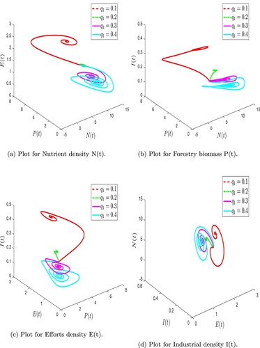
Figure 16. Numerical simulation of forestry biomass model (31(31) $\begin{array}{rl}{}^{\mathrm{FFP}}{}_{0+}{\mathfrak{D}}_t^{\psi ,\phi }N\left(t\right)& =Q-\text{β}P-d_{1}N,\\ {}^{\mathrm{FFP}}{}_{0+}{\mathfrak{D}}_t^{\psi ,\phi }P\left(t\right)& =r\left(N\right)P(1-\frac{P}{K})-q_1\mathrm{PE}-d_2\mathrm{PE}+\mathrm{\gamma P},\\ {}^{\mathrm{FFP}}{}_{0+}{\mathfrak{D}}_t^{\psi ,\phi }E\left(t\right)& =q_1(p-\tau )\mathrm{PE}+p{d}_2\mathrm{PE}-\mathrm{cE},\\ {}^{\mathrm{FFP}}{}_{0+}{\mathfrak{D}}_t^{\psi ,\phi }I\left(t\right)& =\mathrm{\alpha E}+\mathrm{\mu I}(1-\frac{P}{K})-d_{3}I.\end{array}$(31) ) at arbitrary values of $q_1$ with $\psi =0.99$. (a) Plot for Nutrient density N(t). (b) Plot for Forestry biomass P(t). (c) Plot for Efforts density E(t) and (d) Plot for Industrial density I(t).

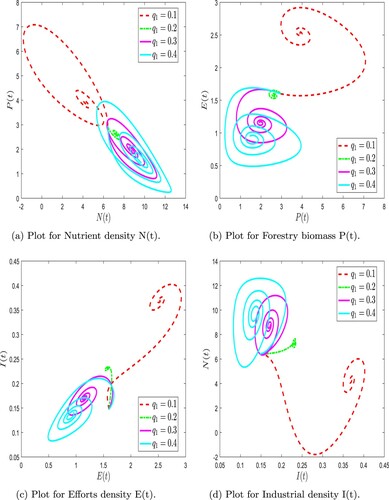
Figure 17. Numerical simulation of forestry biomass model (31(31) $\begin{array}{rl}{}^{\mathrm{FFP}}{}_{0+}{\mathfrak{D}}_t^{\psi ,\phi }N\left(t\right)& =Q-\text{β}P-d_{1}N,\\ {}^{\mathrm{FFP}}{}_{0+}{\mathfrak{D}}_t^{\psi ,\phi }P\left(t\right)& =r\left(N\right)P(1-\frac{P}{K})-q_1\mathrm{PE}-d_2\mathrm{PE}+\mathrm{\gamma P},\\ {}^{\mathrm{FFP}}{}_{0+}{\mathfrak{D}}_t^{\psi ,\phi }E\left(t\right)& =q_1(p-\tau )\mathrm{PE}+p{d}_2\mathrm{PE}-\mathrm{cE},\\ {}^{\mathrm{FFP}}{}_{0+}{\mathfrak{D}}_t^{\psi ,\phi }I\left(t\right)& =\mathrm{\alpha E}+\mathrm{\mu I}(1-\frac{P}{K})-d_{3}I.\end{array}$(31) ) at arbitrary values of $q_1$ with $\psi =0.99$. (a) Plot for Nutrient density N(t). (b) Plot for Forestry biomass P(t). (c) Plot for Efforts density E(t) and (d) Plot for Industrial density I(t).

Data availability statements

Data available on request from the authors.